Electricity has a rather unreasonable requirement.
At every moment, the amount of electricity entering the power system has to match the amount leaving it.
Not approximately.
Not by the end of the month.
Not after accounting closes on Friday.
Now.
A power plant trips.
A steel mill starts a furnace.
A cloud passes over a solar farm.
The wind forecast misses by 500 MW.
Millions of people simultaneously decide that 7 p.m. is an excellent time to cook dinner.
The power system cannot respond:
“We’ll reconcile that tomorrow.”
Tomorrow is far too late.
Welcome to 1000whats – where today we look at one of the most fundamental jobs in the electricity system:
keeping production and consumption in balance while both are constantly changing.
That job is called:
electricity balancing.
And before we talk about balancing markets, imbalance prices, BRPs, BSPs or any of the other acronyms the industry has generously prepared for us, we need to understand the physical problem.
Fortunately, the physical problem is beautifully simple.
Electricity starts with a plan
Tomorrow’s electricity system is not improvised tomorrow.
Generators prepare schedules.
Suppliers forecast consumption.
Wind and solar producers forecast production.
Market participants buy and sell electricity.
System operators prepare for the expected operating conditions.
By the time a particular delivery period arrives, the power system has a very detailed idea of what is supposed to happen.
Take a simplified generator.
Based on historical production and its forecast, it prepares the following schedule for tomorrow.
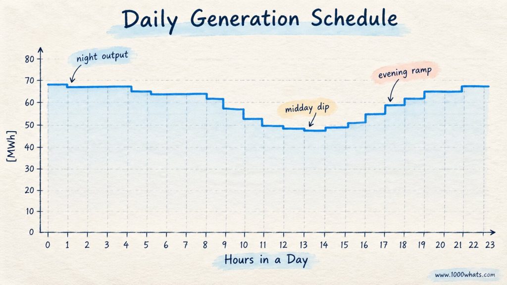
This first diagram looks almost boring.
That is exactly what we want.
The horizontal axis shows the hours of the day.
The vertical axis shows scheduled production.
Our generator expects to produce roughly 68 MW during the night. Production gradually falls toward about 48 MW around midday, then rises again toward the evening.
Each step represents the amount of electricity the generator expects to inject during that period.
At this stage, there is no imbalance.
There is no emergency.
There is no balancing action.
There is simply:
a plan.
⚡ “Electricity balancing begins with a surprisingly ordinary idea: first decide what you expect to happen.”
Of course, an actual power system contains thousands of such plans.
Generators have schedules.
Consumption has forecasts.
Cross-border exchanges have schedules.
Storage may be charging or discharging.
Put all of that together and the system operator enters real time expecting a particular relationship between generation, consumption and scheduled exchanges.
Then real time arrives.
And reality begins editing the spreadsheet.
The orange line ruins everything
Here is the same generator the following day.
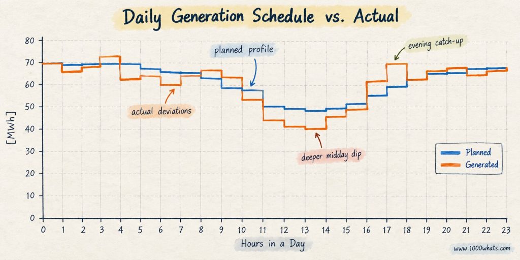
Blue is what it planned to produce.
Orange is what it actually produced.
Now the interesting part begins.
At midnight, the generator planned about:
68 MW
and produced:
68 MW.
Blue and orange sit on top of each other.
Nothing to see.
A little later, actual generation falls below the schedule.
Suppose the plant was scheduled at:
67 MW
but actually produced:
64 MW.
The difference is:
-3 MW.
Later, the opposite happens.
Scheduled production might be:
62 MW
while actual production reaches:
66 MW.
Difference:
+4 MW.
And around midday the deviation becomes much larger.
The blue line says roughly:
49 MW.
The orange line falls to around:
40 MW.
That missing production is no longer a forecast problem.
It is physically happening.
This is the first concept we need:
a schedule and physical delivery are not the same thing.
The schedule says what should happen.
The meter eventually tells us what did happen.
The difference between them is a deviation.
And deviations are unavoidable.
Why is actual generation different from the schedule?
For a conventional generator, perhaps:
a unit trips,
output is constrained,
equipment behaves differently than expected,
or operating conditions change.
For wind:
the wind forecast was wrong.
For solar:
cloud cover developed differently.
For hydro:
water availability or operating decisions changed.
Consumption is even more entertaining.
Nobody submits a form before turning on an oven.
Millions of individual decisions combine into system demand, and system operators forecast the result remarkably well.
But remarkably well is not:
perfectly.
Forecast errors are therefore not evidence that somebody has failed to understand electricity.
They are a normal feature of operating a system whose future is uncertain.
The balancing problem exists because:
plans are discrete and knowable. Reality is continuous and slightly rude.
Now look at the space between the lines
The next version of your diagram makes the concept much easier to see.
We keep:
the blue scheduled-production line
and:
the orange actual-production line.
But now we explicitly show the difference between them.
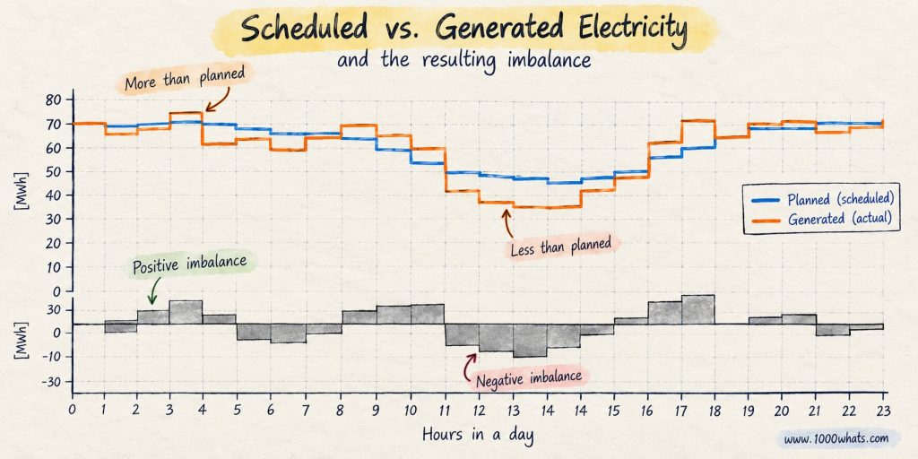
This is one of the diagrams I would make central to the article.
Read it from top to bottom.
The blue staircase is still the schedule.
The orange staircase is actual generation.
The gray bars underneath represent the deviation.
Where orange is below blue, the generator has produced less than scheduled.
Where orange is above blue, it has produced more than scheduled.
At around midday, for example, the scheduled value is roughly 49 MW while actual generation drops to about 40 MW.
The deviation is therefore roughly:
-9 MW.
That gray bar is not another mysterious electricity product.
It is simply:
the gap between the two lines.
That is the visual idea I want readers to remember.
No balancing-market terminology yet.
No settlement formula.
Just:
blue – what we expected
orange – what happened
gray – the difference
Once that clicks, half of balancing becomes much easier to understand.
A tiny numerical example
Suppose one generator has:
Scheduled production = 100 MW
Actual production = 92 MW
Deviation:
92 – 100 = -8 MW
Another generator has:
Scheduled production = 80 MW
Actual production = 85 MW
Deviation:
85 – 80 = +5 MW
Meanwhile demand turns out:
4 MW higher than expected.
Now things become interesting.
Because the power system does not care only about the deviation of one generator.
It cares about:
the net result of everything happening at once.
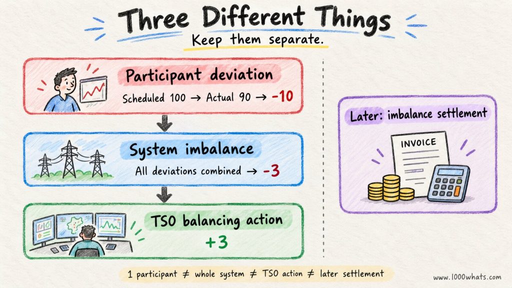
One generator’s deviation is not the system imbalance
This distinction is crucial.
Our orange and blue diagram shows the deviation of one participant or one portfolio.
That is not automatically the imbalance of the entire power system.
Imagine:
Wind farm A: -100 MW
Solar plant B: +30 MW
Generator C: +20 MW
Demand: 10 MW lower than expected
Those deviations partially cancel.
Net result:
-100 + 30 + 20 + 10 = -40 MW
The wind farm missed its schedule by 100 MW.
But the system is not necessarily 100 MW short.
It is:
40 MW short.
This is why looking at one generator tells you something about that generator.
Looking at the aggregate tells you what the system operator has to deal with.
And sometimes the opposite happens.
Several individually small deviations all point in the same direction.
Suddenly the system has a large problem even though nobody individually did anything dramatic.
⚡ “The grid does not balance every forecast error separately. It balances the net physical result of all of them happening at the same time.”
That sentence is important.
It separates portfolio deviation from system balancing.
Later, when we get to imbalance settlement, this distinction will become even more important.
But not today.
Today we stay with physics.
What happens if the system is short?
Suppose total electricity consumption is:
10,000 MW.
But generation and net imports currently provide only:
9,900 MW.
The system is short:
100 MW.
That missing 100 MW cannot simply remain missing.
In an AC power system, an active-power imbalance shows up in the behavior of system frequency.
If consumption exceeds generation, frequency tends to fall.
If generation exceeds consumption, frequency tends to rise.
My article on grid inertia explains the immediate physical response in more detail.
But there is an important nuance.
Balancing is not simply “watch frequency and turn generators up until it says 50 Hz.”
In a large interconnected synchronous system such as Continental Europe, frequency is shared across an enormous area.
Individual control areas also have scheduled exchanges with their neighbors.
A TSO therefore has to restore not only frequency but also its area’s power balance relative to scheduled exchanges.
ENTSO-E’s framework distinguishes these layers explicitly: Frequency Containment Reserve first stabilizes frequency after an imbalance, while Frequency Restoration Reserves subsequently restore frequency and, in multi-area synchronous systems, restore the affected control area’s power balance toward its scheduled value.
That sounds technical.
The simple version is:
the whole interconnected system initially feels the disturbance, but the area that caused it ultimately has to clean up after itself.
Electricity has neighbors.
They may help when you drop a plate.
They do not want to spend the rest of the evening holding your broom.
The first response happens almost immediately
Suppose a 1,000 MW power plant suddenly trips.
Generation instantly falls by:
1,000 MW.
Demand has not politely fallen by 1,000 MW at exactly the same moment.
So:
generation < demand.
For the first moments, stored kinetic energy in rotating machines helps resist the frequency change.
Then frequency containment reserves respond.
Their immediate job is:
stop the fall.
Not necessarily return everything instantly to the original condition.
Stop the deterioration first.
Think of a car beginning to roll downhill.
The first job is the brake.
Returning the car neatly to its original parking spot comes later.
This is why my existing article on ancillary services separates the sequence of frequency-control services rather than treating “reserve” as one giant emergency button.
Then somebody has to restore the balance
Stabilizing frequency is not the end of the story.
The missing power still has to be replaced.
That is where frequency restoration enters.
Resources can:
increase generation,
reduce generation,
increase consumption,
reduce consumption,
charge storage,
or discharge storage,
depending on which direction the system needs to move.
If the system is short, it needs upward balancing.
That could mean:
- a hydro plant increases production;
- a gas plant ramps upward;
- a battery discharges;
- an industrial consumer reduces demand.
If the system is long, it needs downward balancing.
That could mean:
- a generator reduces production;
- a battery starts charging;
- flexible consumption increases;
- renewable output is reduced where appropriate.
Notice something important.
Balancing does not inherently mean:
start another power plant.
A 50 MW increase in generation and a 50 MW reduction in consumption have the same first-order effect on the active-power balance.
One adds 50 MW on one side.
The other removes 50 MW from the other.
The grid is remarkably uninterested in the philosophical difference.
Now look at what balancing looks like in the real world
This is where I would use your strongest real-data diagram.
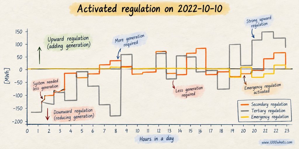
The chart below is based on actual activated regulation in Serbia on October 10, 2022.
And I would explain this diagram carefully, because it is fantastic.
At first glance it looks chaotic.
Good.
Balancing is chaotic compared with a nice smooth daily schedule.
The horizontal axis again shows the day.
But now the vertical axis shows activated balancing energy in either direction.
Three different types of regulation are visible in the original data:
secondary regulation
tertiary regulation
and occasional:
emergency regulation.
Look first at the left side of the graph.
During the early hours, much of the activated regulation is below zero.
That means the system required balancing in one direction.
Later, the sign changes.
Around hours 11-12, substantial regulation appears in the opposite direction.
Then it changes again.
And again.
By the evening, tertiary regulation reaches well above:
100 MWh in some accounting intervals.
This is the real point of the graph.
Balancing is not:
“Tomorrow we expect to be 200 MW short, so please start Generator X.”
That is scheduling.
Balancing is what happens after reality starts deviating from those schedules.
The direction can change.
The required volume can change.
Different resources can respond.
One interval can require downward regulation.
A later interval can require upward regulation.
Sometimes both secondary and tertiary resources are involved.
On this particular day, emergency regulation also appears in several periods.
The grid is continuously correcting itself.
Not because somebody planned badly once.
Because the target itself is moving while thousands of physical variables are moving around it.
This graph is essentially the heartbeat of balancing.
But where did those balancing megawatts come from?
Now we deliberately stop.
Because this is exactly where the next article begins.
The TSO does not own some magical warehouse containing spare electricity.
The ability to move generation, storage or consumption has to come from physical resources.
Those resources must be:
available,
technically capable,
controllable,
and under modern arrangements often commercially offered to the TSO.
Who provides them?
How do they qualify?
How much capacity is reserved?
How is balancing energy offered?
Which bid gets activated?
What is a BSP?
Why are there separate aFRR and mFRR products?
How do PICASSO and MARI fit into this?
Those are questions about the:
balancing market.
And they deserve their own article.
For now, we need only understand what that market exists to solve.
A physical imbalance.
Balancing is not the same as being balanced
This distinction will save us considerable confusion later.
A market participant may be:
in imbalance.
The power system is:
being balanced.
Those are not the same statement.
Suppose a wind producer generates 20 MWh less than its final position.
Somebody else happens to produce 15 MWh more.
Consumption comes in 3 MWh lower.
The system operator may ultimately need only a small additional correction.
Later, the market operator or settlement function will determine:
who deviated,
by how much,
at what imbalance price,
and who owes whom money.
That is:
imbalance settlement.
We are deliberately not solving it here.
Because physical balancing happens in real time.
Financial settlement happens afterward.
Confusing the two is one of the fastest ways to make electricity balancing look much more mysterious than it really is.
So why bother with schedules at all?
There is an obvious question.
If balancing exists because schedules will inevitably be wrong, why make schedules?
Because balancing is supposed to correct:
the residual error.
Not run the entire electricity system from scratch.
Imagine running a restaurant with no reservations, no food inventory, no staff schedule and no idea how many customers are coming.
Then keeping 40 emergency chefs outside in case dinner becomes unexpectedly popular.
Technically flexible.
Commercially insane.
The electricity system does the opposite.
Forecast as well as possible.
Schedule production and consumption.
Trade electricity.
Update forecasts.
Adjust positions closer to delivery.
Then use balancing resources for what remains.
The better the system gets at forecasting and short-term adjustment, the smaller the residual balancing problem can become.
But it will never become zero.
A power system with perfect forecasts would still experience:
plant trips,
network disturbances,
unexpected demand changes,
equipment failures,
and other events that occur after the forecast has finished being useful.
Balancing is therefore not a temporary patch until forecasting gets better.
It is a permanent feature of electricity.
The system can also be balanced while individual participants are wrong
This is another beautifully counterintuitive point.
Imagine two wind farms.
Wind Farm A scheduled:
100 MW
and produces:
80 MW.
Deviation:
-20 MW.
Wind Farm B scheduled:
100 MW
and produces:
120 MW.
Deviation:
+20 MW.
Individually:
both are wrong.
Together:
zero.
From the system’s active-power balance perspective, their deviations cancel.
Now imagine both produce:
80 MW.
Each is:
-20 MW.
Together:
-40 MW.
Same individual forecast error.
Completely different system consequence.
That is why the direction of an individual imbalance matters.
But the system direction matters too.
And that distinction will become very important when we eventually discuss imbalance pricing.
For now, remember:
being wrong is not exactly the same thing as making the system worse.
That sentence will come back later.
What does frequency have to do with all of this?
Frequency is the physical messenger.
In Continental Europe, nominal frequency is:
50 Hz.
When generation and consumption move out of balance, frequency responds.
Too little generation relative to demand:
frequency tends to fall.
Too much generation:
frequency tends to rise.
This makes frequency an extraordinarily useful system-wide indicator.
But frequency should not be confused with the accounting concept of imbalance.
A generator can have a commercial deviation from its schedule while system frequency remains very close to 50 Hz because other deviations and balancing actions offset it.
Conversely, a sudden major generator trip can create a system-wide frequency disturbance before anyone has had time to calculate an imbalance invoice.
One belongs first to:
physics.
The other also belongs to:
market accounting.
They interact.
They are not synonyms.
The hierarchy now becomes surprisingly simple
We can finally assemble the whole story.
Before delivery:
we make a plan.
During delivery:
reality deviates from the plan.
Across the whole system:
those deviations combine into a system imbalance.
Physics reacts:
frequency and scheduled area exchanges begin to reflect that imbalance.
Fast reserves stabilize the system.
Balancing resources then:
increase or decrease net power to restore balance.
Later:
market and settlement mechanisms determine:
who provided the balancing service and who was financially responsible for imbalances.
That last sentence contains two completely different economic questions.
Which is why we are giving each one its own article.
⚡ “Balancing is not an accounting exercise. The accounting exists because somebody had to physically balance the grid first.”
What changes with more wind, solar and batteries?
Balancing is sometimes presented as a problem invented by renewable energy.
It was not.
Power systems required balancing when almost every major generator burned coal.
A 1 GW thermal unit can disappear from the system in seconds.
Demand has never been perfectly predictable.
Transmission systems have never been immune to disturbances.
What wind and solar change is the nature and distribution of uncertainty.
Weather-dependent production creates additional forecast variability.
At the same time, the resources available for balancing are changing.
Historically, balancing was heavily associated with controllable conventional and hydro generation.
Now it can increasingly come from:
batteries,
demand response,
aggregated distributed resources,
renewable generators,
cross-border resources,
and combinations of them.
ENTSO-E explicitly describes the European balancing framework as both a way to maintain generation-demand balance and a mechanism for opening participation to resources such as demand response and renewables.
The balancing problem remains.
The toolbox is changing.
And neighboring countries can help
One final idea prepares us for later in the series.
Imagine Serbia needs:
+100 MW.
A neighboring control area simultaneously needs:
-80 MW.
One system needs more net power.
The other needs less.
Activating +100 MW in one country and -80 MW in the other would be rather enthusiastic.
If the systems and market arrangements allow those opposite needs to offset, much of the required activation can disappear.
ENTSO-E calls this imbalance netting: TSOs can avoid simultaneous frequency-restoration activations in opposite directions by accounting for opposing control-area needs.
In our simplified example:
+100 MW
and:
-80 MW
leave only:
+20 MW
to solve.
Sometimes the cleverest balancing action is:
not activating two balancing actions that cancel each other.
We will come back to that.
Europe has built an increasingly elaborate cross-border architecture around exactly this idea.
What is electricity balancing in one sentence?
Electricity balancing is the continuous process of correcting differences between electricity generation and consumption so the power system remains physically balanced in real time.
But I prefer the visual definition.
Remember our diagram.
Blue line: what we planned.
Orange line: what actually happened.
Then zoom out from one generator to the entire power system.
Combine thousands of differences.
What remains is the problem the TSO has to solve.
That:
is balancing.
Final thoughts
Electricity balancing sounds complicated because the industry surrounds it with:
FCR,
aFRR,
mFRR,
BRPs,
BSPs,
ISPs,
imbalance prices,
balancing platforms,
control areas,
merit-order lists,
and enough regulation to support a medium-sized legal ecosystem.
We will get to all of that.
But none of it is the fundamental idea.
The fundamental idea fits on one Excel chart.
We planned one line.
Reality produced another.
Across an entire power system, all those little differences combine into a physical result.
And electricity has one uncompromising rule:
somebody has to close the gap.
Immediately.
That is electricity balancing.
The next question is obvious.
Who is willing and able to move generation or consumption when the TSO needs it – and how does the TSO choose between them?
That is where physics becomes a market.
And that is our next article:
What Is a Balancing Market?
Until next time, stay curious! 😎
Discover more from 1000whats
Subscribe to get the latest posts sent to your email.