
The restaurant has served 1,000 dinners. The kitchen has roasted vegetables, baked bread, simmered soup, and persuaded a large industrial dishwasher to keep its opinions to itself.
At closing time, the manager adds up the kitchen’s expenses and announces an average cost of $12 per meal.
Then you arrive, seventeen minutes late, and order a steak.
The vegetables are gone. The ovens are cooling. To serve you, the chef must fire up a gas grill, call back a cook, and reopen a kitchen that was already dreaming of tomorrow.
The manager looks at your order and says, “That will cost us $12. It’s the average.”
The chef puts down the tongs very carefully.
Electricity has a similar accounting problem, except the kitchen covers a continent, the menu changes every few minutes, and the customers keep ordering while the chefs are trying to replace the stove.
A grid can have a perfectly accurate average carbon intensity and a very different marginal emissions factor. One tells us how much pollution to allocate across the electricity already produced. The other estimates what happens to emissions when demand or generation changes.
Both are useful. Confusing them is how a reasonable-looking spreadsheet can reach a thoroughly unreasonable conclusion.
Welcome to 1000whats, where the electricity bill has acquired a second receipt, and the second one is considerably more argumentative.
The average receipt is honest. It is answering a different question.
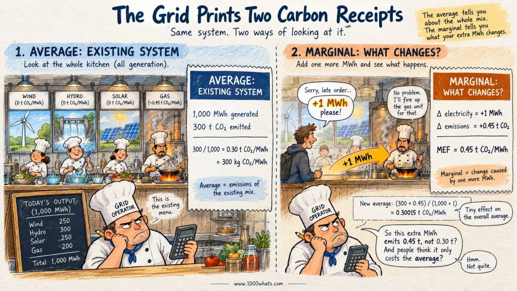
Suppose a power system produces 1,000 megawatt-hours (MWh) of electricity during a particular period and its power plants emit 300 metric tons of CO₂.
The average operational emissions rate is:
300 t CO₂ ÷ 1,000 MWh = 0.30 t CO₂/MWh.
That’s 300 kilograms of CO₂ per MWh, or 300 grams per kWh. Same number, different outfit.
It is a sensible description of the electricity mix. Nuclear, hydro, wind, solar, gas, coal, and whatever else generated during the period all contribute to the denominator; direct emissions from the relevant power plants contribute to the numerator. Boundaries and accounting conventions matter, but the arithmetic is uncomplicated.
If you want the fuller picture of that calculation, my guide to carbon intensity covers the foundations.
Now imagine an additional customer requests 1 MWh of electricity during that same period. The operator responds by increasing the output of a gas-fired unit, whose incremental direct CO₂ emissions are 0.45 t for that extra MWh.
The extra electricity causes approximately 0.45 t CO₂ of additional power-plant emissions, not 0.30 t. In this deliberately simplified example, the new system average becomes:
(300 + 0.45) t ÷ (1,000 + 1) MWh ≈ 0.30015 t CO₂/MWh.
The average barely moves. The incremental consequence is still 0.45 t.
That is the entire intellectual troublemaker hiding behind the phrase marginal emissions factor.
An average tells you how the existing emissions are distributed. A marginal factor asks what emissions change when you change the system.
Neither number is a correction of the other. They’re answering different questions. Asking the average to predict an incremental change is like using the restaurant’s average dinner cost to decide whether reopening the grill for one late steak is a bargain.
So what exactly is a marginal emissions factor?
A marginal emissions factor (MEF) estimates the change in emissions caused by a change in electricity demand, supply, or another specified intervention, within a defined place, period, and set of assumptions.
In compact form:
Marginal emissions factor ≈ Change in power-system emissions ÷ Change in electricity supplied or consumed.
For a small increase in demand, that can be written as ΔCO₂ / ΔMWh. The unit is typically kg CO₂/MWh, t CO₂/MWh, or the equivalent in CO₂e if the analysis includes other greenhouse gases using a specified global-warming-potential convention.
Notice the word change. We are comparing two situations: the system as it would operate without your intervention, and the system as it would operate with it. That missing alternative is called the counterfactual. Without one, the carbon receipt has no meaningful second column.
For a sufficiently small change, a local marginal factor can be useful. For a large intervention, however, the response may not be linear. A 1 MWh increase and a 1,000 MWh increase can trigger entirely different plants, transmission flows, starts, shutdowns, and constraints.
So 1,000 × the one-MWh marginal factor is not automatically a reliable estimate of the impact of 1,000 MWh. The chef might buy another oven before accepting that order.
A marginal factor is not a permanent property of a fuel or a country. It is a property of a system response under specified conditions.
Why the last power plant is not always the whole story
A popular shortcut says that the marginal emissions factor belongs to the “last power plant” dispatched. It’s a helpful first mental picture, but reality has an unfortunate habit of reading the footnotes.
In a simplified competitive power market, plants offer electricity according to their costs and operating conditions. Lower-cost resources tend to be dispatched first, while higher-cost resources may be needed as demand increases. My explanation of the merit order shows how that queue works.
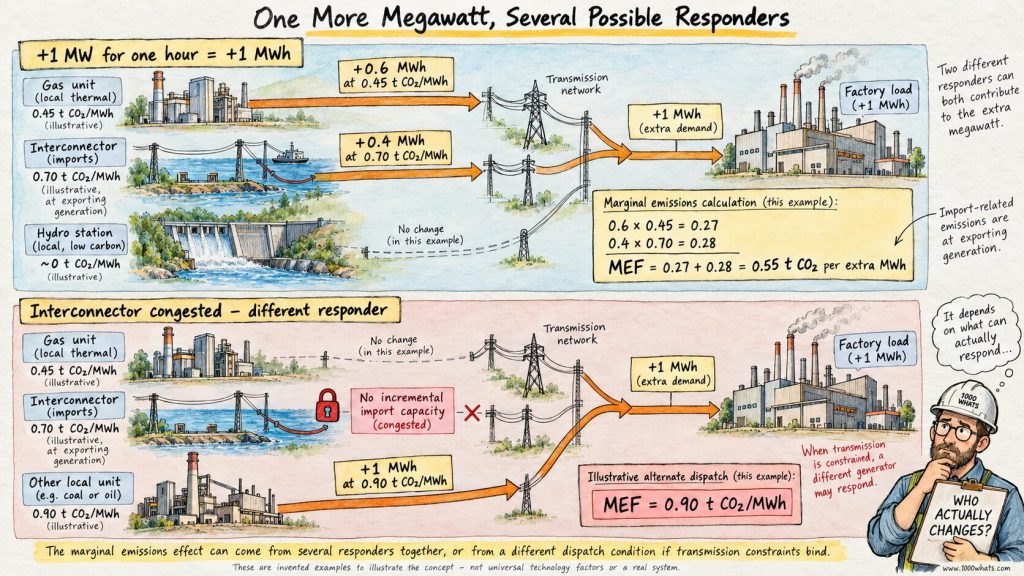
If a gas plant is the unit that can increase output by 1 MW, it may be the marginal responder. But it could also be a hydro plant, an import, a battery, or a combination of resources. Some plants cannot ramp quickly. Others have minimum stable output, startup costs, fuel constraints, or obligations to provide reserves.
And power does not travel according to the preferences of the nearest spreadsheet. Transmission congestion can make a generator across the border irrelevant to the extra demand at your particular location, even if that generator is cheap and clean.
In more sophisticated analyses, the response to a small load change is distributed across several units. The marginal factor then reflects the combined change in emissions, not a photograph of one heroic generator wearing a sash labeled MARGINAL.
Even the phrase “last plant” can mislead when the response involves less curtailment, changed imports, altered storage dispatch, or a generator that must start for several hours to cover a brief demand increase.
The question is not “Which plant has the highest operating cost?” It is “Which operating decisions change because this intervention happens?”
That distinction is what turns a dispatch story into an emissions calculation.
Two receipts, side by side
Here is the practical difference between the two numbers.
| Question | Average emissions factor | Marginal emissions factor |
|---|---|---|
| What does it describe? | Emissions attributed to electricity in a defined mix and period | Emissions changed by an additional or avoided amount of electricity |
| Typical calculation | Total emissions ÷ total electricity | Change in emissions ÷ change in electricity |
| Main use | Inventories, attribution, comparisons of electricity mixes | Evaluating operational decisions and avoided-emissions impacts |
| Does timing matter? | Yes, if using time-specific averages; annual averages conceal hourly variation | Often critically, because the responding resources change over time |
| Can it identify a causal impact by itself? | No | It estimates one, subject to model assumptions and system boundaries |
| Is one always larger? | No | No; it may be above, below, or near the average |
There is a particularly sneaky trap here: an hourly average is still an average. Replacing a yearly carbon-intensity figure with 8,760 hourly figures improves temporal detail, but it does not magically turn an attributional measure into a marginal one.
If every generator’s emissions are averaged over an hour, that is still the kitchen’s average bill for that hour. It does not tell you which burner responds to the next order.
The lunchtime surprise: sometimes extra demand adds almost no emissions
Let’s give the chef a break and send the electricity system some sunshine.
Imagine a sunny afternoon with so much available solar generation that part of it would otherwise be curtailed. A flexible industrial process switches on and uses 1 MWh of electricity that, without that process, could not have been exported or stored and would have gone unused.
Under those specific assumptions, the additional demand may simply reduce solar curtailment by 1 MWh. The immediate incremental operational CO₂ emissions from generation could be close to zero.
The average electricity mix during that same hour might still include gas and coal. Its average carbon intensity could therefore be substantially above zero.
Now move the identical industrial process to an evening hour when the system needs an additional fossil-fired unit. The same 1 MWh of consumption could cause a much larger emissions increase.
Same machine. Same energy. Same factory manager claiming that the shift schedule was already complicated enough.
Different consequence.
But “solar is available” is not the same as “solar is marginal.” If available solar is already fully used, more demand may increase fossil generation or imports. If a network constraint prevents the surplus from reaching the load, the hypothetical zero-emissions opportunity may not exist at that location. If a battery would otherwise have charged from the surplus and displaced fossil generation later, consuming it now can carry an opportunity cost.
The marginal answer depends on what would have happened otherwise, not on the presence of sunshine in a stock photograph.
This is why my article on curtailment is relevant: electricity that could have been generated is not necessarily electricity the system can use.
One factory, three hours, three very different answers
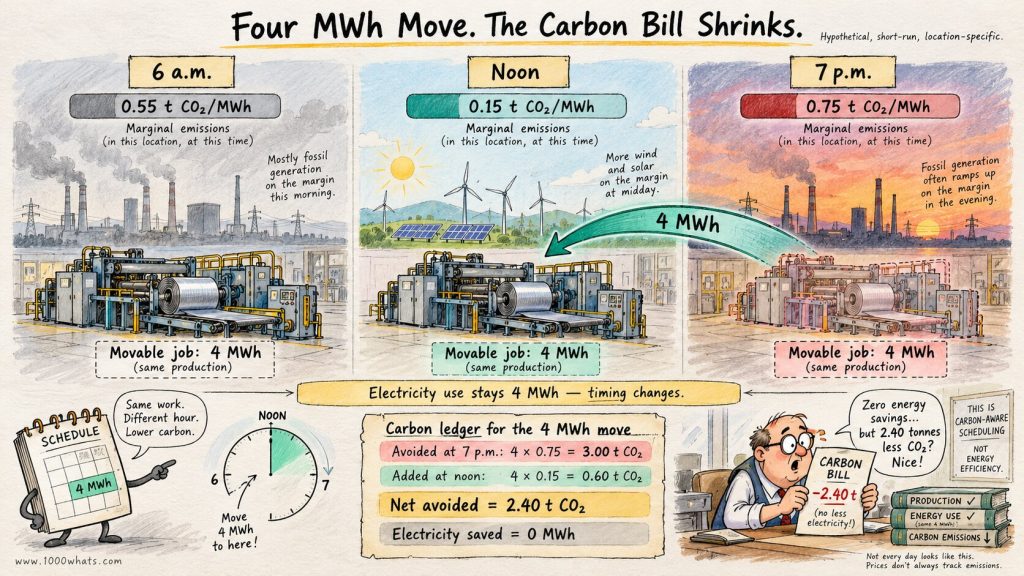
Consider an illustrative grid with the following estimated short-run marginal CO₂ rates. These are invented teaching values, not observed data for any country, year, or balancing area.
| Hour and assumed system condition | Estimated marginal CO₂ rate | Incremental emissions from 1 MWh |
|---|---|---|
| 6 a.m., flexible gas generation responding | 0.55 t CO₂/MWh | 0.55 t CO₂ |
| Noon, a low-emissions combination of resources responds | 0.15 t CO₂/MWh | 0.15 t CO₂ |
| 7 p.m., a higher-emitting resource responds | 0.75 t CO₂/MWh | 0.75 t CO₂ |
Suppose a factory can move a production batch requiring 4 MWh from the evening period to noon, without changing production, energy consumption, or any other system behavior.
In this simplified calculation, the avoided evening emissions are:
4 MWh × 0.75 t CO₂/MWh = 3.00 t CO₂.
The additional noon emissions are:
4 MWh × 0.15 t CO₂/MWh = 0.60 t CO₂.
The estimated net reduction is:
3.00 − 0.60 = 2.40 t CO₂.
The factory has saved zero MWh. Its total electricity consumption is unchanged. Yet, under our assumptions, the grid emits 2.40 fewer tons of CO₂.
The finance director may also see a lower electricity bill if noon prices are lower, but that is a separate calculation. Carbon savings are not printed on the wholesale price tag.
This is the emissions side of energy arbitrage and demand shifting. The electricity moves through time; the environmental outcome depends on what that movement displaces.
A caution: the example treats marginal rates as constant across the shifted 4 MWh and ignores process losses, rebound, grid constraints, and changes in unit commitment. Real project analysis must test those assumptions. Our little factory is a classroom, not a certified carbon-credit factory.
Batteries: the carbon accountant discovers round-trip efficiency
A battery adds a wonderfully inconvenient detail. It cannot deliver every MWh it charges with. Some energy becomes heat, and the laws of thermodynamics decline to issue refunds.
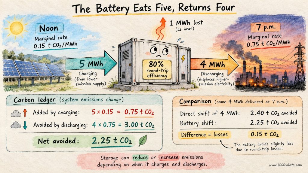
Suppose a battery delivers 4 MWh during the 7 p.m. period in our example. Its round-trip efficiency is 80%. To deliver those 4 MWh, it must have charged with approximately:
4 MWh ÷ 0.80 = 5 MWh.
At the illustrative noon marginal rate of 0.15 t CO₂/MWh, charging adds:
5 × 0.15 = 0.75 t CO₂.
At the evening rate of 0.75 t CO₂/MWh, discharging displaces:
4 × 0.75 = 3.00 t CO₂.
So the estimated net reduction is:
3.00 − 0.75 = 2.25 t CO₂.
The battery can help, despite losing 1 MWh in the process. It is moving energy from a lower-emissions hour to a higher-emissions hour, and the difference is large enough to overcome its losses.
But reverse the emissions conditions and the same battery could increase operational emissions. Charging from a high-emissions marginal resource and displacing a cleaner one later is not a climate victory merely because the battery has a green icon on the control screen.
The simplified equation for this kind of energy shift is:
Net avoided emissions ≈ Discharged MWh × marginal rate at discharge − Charged MWh × marginal rate at charge.
This is a short-run operational calculation. A fuller study may include degradation, auxiliary electricity, battery manufacturing, alternative uses of stored energy, and the way repeated storage operation changes the market itself.
The U.S. Environmental Protection Agency’s AVERT tool is one example of a framework designed to estimate how interventions, including storage and clean energy, change power-sector emissions. It is not a universal carbon calculator for every grid on Earth.
Electricity crosses borders. So do the consequences.
Suppose your factory is in Country A. It increases electricity demand, and the balancing area responds by importing an extra MWh from Country B.
Whose emissions should the marginal analysis count?
If the intervention causes a power plant in Country B to increase generation, the causal emissions effect may occur there. Restricting the calculation to smokestacks physically located in Country A would miss it.
Now add congestion. Perhaps the interconnector is full. Perhaps an additional import is impossible, so a local unit must respond instead. Perhaps a dispatch change in one area reduces exports from another, creating a chain of responses.
A country’s average generation mix is not necessarily the mix supplying its consumers, and neither is automatically the marginal response to extra demand. This is why production-based, consumption-based, and consequential perspectives must be distinguished.
A useful marginal model needs a realistic electrical boundary, transmission constraints, trade assumptions, and the right time resolution. The electricity system is physically interconnected; national borders are excellent at organizing paperwork but less talented at instructing alternating current where to stop.
Cheap electricity is not automatically clean electricity
Here is another tempting shortcut: just charge batteries or run factories whenever electricity prices are lowest. Surely the cheapest hours are also the cleanest?
Sometimes. Not always.
A low price can signal abundant wind or solar, which may coincide with low marginal emissions. It can also reflect demand conditions, inflexible conventional generation, transmission constraints, or market arrangements that do not map neatly onto the emissions of the resources responding to a small change.
Conversely, an expensive hour might have hydroelectric generation on the margin, or scarce low-carbon flexibility, while a cheaper hour elsewhere relies on fossil generation.
Wholesale prices are formed from bids, offers, network constraints, and market rules. Marginal emissions come from the physical changes in generation and operation that an intervention causes. Related mechanisms, different questions.
The merit-order curve can help you understand price formation. It cannot, by itself, issue a reliable carbon receipt. A dispatchable unit’s short-run cost and its CO₂ emissions are not the same variable.
For serious scheduling decisions, compare hourly prices and hourly marginal emissions estimates separately. A project may pursue both cost and emissions objectives, but the cheapest operating schedule is not guaranteed to be the cleanest.
The corporate carbon accountant is not wrong, either
At this point, someone from the sustainability department usually raises a hand.
“Our company’s electricity footprint uses an average emissions factor. Are you saying our inventory is wrong?”
No. Please put down the spreadsheet. Nobody is confiscating it.
A corporate emissions inventory asks a different question from an avoided-emissions study. An inventory allocates responsibility for emissions associated with a company’s activities according to an established accounting framework. A consequential study asks how emissions would change if the company took a particular action.
The GHG Protocol Scope 2 Guidance distinguishes two principal methods for reporting emissions from purchased electricity and other acquired energy:
- Location-based: uses emission factors reflecting the average emissions intensity of electricity associated with a defined location, generally within the prescribed geographic and temporal boundary.
- Market-based: uses qualifying contractual instruments and related emissions information to reflect the attributes of electricity a company has contractually purchased or claimed, following the standard’s quality criteria.
A marginal factor is not a substitute for the required location-based Scope 2 factor. Nor can a company simply deduct a modeled avoided-emissions estimate from its inventory and announce that the remainder is its official footprint.
That would be like using the money saved by cancelling tomorrow’s dinner reservation to rewrite the receipt for last night’s meal. Both amounts matter. They belong in different columns.
Here is the distinction in one place:
| Decision or reporting task | More appropriate starting point | Important qualification |
|---|---|---|
| Report location-based purchased-electricity emissions | Applicable average grid factor | Follow the relevant Scope 2 rules and geographic boundary |
| Report market-based purchased-electricity emissions | Qualifying contractual attributes and factors | Follow certificate, residual-mix, and quality criteria |
| Estimate emissions avoided by shifting a flexible load | Time- and location-specific marginal estimates | Compare the counterfactual schedules and include losses |
| Estimate the impact of a major new industrial facility | Forward-looking system modeling | Account for new generation, network, and demand response over time |
| Compare operational and life-cycle climate impacts | Boundary-specific life-cycle analysis | Do not mix stack CO₂ with cradle-to-grave CO₂e |
Both kinds of information can support better decisions. The mistake is treating them as interchangeable because both use the letters CO₂ and arrive in an Excel cell.
A renewable certificate does not change the physical dispatch by magic
Imagine a business purchases renewable electricity certificates covering its annual electricity consumption. Under an applicable market-based accounting method, qualifying certificates may affect the emissions factor used for that company’s reported Scope 2 emissions.
That is a contractual accounting outcome. It does not prove that each hour of the company’s consumption physically caused zero additional emissions at the power plants responding to demand.
Nor does it mean renewable procurement has no real-world benefit. A well-structured long-term procurement arrangement can help finance additional clean generation. The emissions consequences depend on what gets built, what generation is displaced, where, when, and under which counterfactual.
In other words, a certificate is a claim about an attribute under a defined system. A marginal factor is an estimate of a system response. A power purchase agreement can influence both the business and the physical system, but the two effects need to be evaluated on their own terms.
The carbon accountant and the system operator are not enemies. They are two professionals looking at the same grid through different windows, and occasionally wondering why the other one insists on opening a spreadsheet during lunch.
The short run and the long run have different kitchens
So far, we have mostly discussed short-run marginal emissions: what changes when existing power plants, imports, storage, and demand respond to a relatively small intervention under a given fleet and network.
Now imagine a data center announcing a permanent 200 MW load that will operate for twenty years. The power system is not going to treat that demand as an unusually persistent late-night steak order.
Over time, investors may build new generation, retire older units, reinforce transmission, add storage, and change dispatch patterns. Fuel prices and policy can evolve. Demand can move. The grid may become cleaner overall even while the new load increases total electricity consumption.
A long-run marginal emissions analysis tries to capture how an enduring change influences investment and operation, not just tomorrow afternoon’s dispatch.
The distinction matters for electric vehicles, heat pumps, industrial electrification, hydrogen production, and large computing facilities. A short-run factor can answer an immediate operational question. It cannot automatically predict the emissions consequence of an investment that reshapes the system over decades.
For that, analysts may use capacity-expansion and production-cost models, with explicit assumptions about future technology costs, policies, resource availability, and demand.
The National Renewable Energy Laboratory’s study Choosing the Best Carbon Factor for the Job explains why different carbon factors are appropriate for different questions. The important lesson is not that one factor wins. It’s that you should decide what question you are asking before picking the number.
How do analysts estimate marginal emissions in practice?
The quick answer is: with varying degrees of sophistication, and preferably with fewer assumptions hidden behind the word “obvious.”
One approach uses historical relationships between electricity demand and observed power-plant emissions. If regional emissions tend to rise by a certain amount when demand increases, after controlling for relevant factors, that relationship can help estimate a marginal rate. The result depends on the statistical model, data quality, geography, and conditions.
Another approach uses dispatch or production-cost models. The analyst runs the system under a baseline scenario, then runs it again with the proposed change and compares the results. A detailed model may account for generator operating limits, transmission constraints, unit commitment, fuel costs, storage, and cross-border flows.
For longer-term interventions, capacity-expansion models can explore how the generating fleet itself might change.
| Method | Useful for | Main weakness |
|---|---|---|
| Annual grid-average emissions | Attributional overview and inventories | Does not isolate incremental changes |
| Nonbaseload proxy emissions rate | Rapid screening of avoided emissions | Does not identify the actual hourly marginal response |
| Historical statistical marginal estimate | Patterns of short-run response in observed systems | May miss structural changes and unusual conditions |
| Hourly dispatch or production-cost modeling | Operational counterfactuals and network-sensitive changes | Requires detailed assumptions, data, and validation |
| Capacity-expansion plus dispatch modeling | Persistent demand, policy, and investment changes | Sensitive to future scenarios and model design |
In the United States, the EPA’s eGRID guidance distinguishes average output emissions rates from nonbaseload rates, which can serve as a screening proxy for displaced generation. The EPA’s AVERT goes further by estimating changes associated with specified clean-energy and efficiency interventions.
Neither should be mistaken for an infallible real-time sensor that knows the emissions consequences of every individual switch. Models are maps. A map that includes every streetlight would be impressive, but you would still want to check whether the bridge is open.
Five ways to make the carbon receipt lie without changing a single number
The errors are often methodological rather than arithmetic. You can multiply perfectly and still answer the wrong question.
- Use the annual average to estimate a specific hourly intervention. It may be adequate for some inventory purposes, but it cannot reveal the actual response at that hour.
- Assume the marginal unit is always fossil-fueled. Curtailment, hydro, imports, storage, and other responses can change the answer.
- Ignore electricity losses. A MWh delivered to a customer can require more than a MWh generated, depending on network losses and the model boundary.
- Multiply a small-change factor by a massive new load. Large interventions may change which plants run, which assets get built, and even the factor itself.
- Mix CO₂ with CO₂e, or operational with life-cycle emissions. A number describing stack CO₂ cannot be compared directly with a life-cycle greenhouse-gas factor without aligning boundaries and units.
A sixth error deserves honorary membership: pretending uncertainty is an embarrassment. A marginal emissions estimate is only as credible as its counterfactual, assumptions, and sensitivity checks.
When a consultant presents a single factor with six decimal places and no explanation of what it represents, those decimals are not evidence of wisdom. They’re an extremely well-dressed question mark.
Which number should you actually use?
Start with the decision, not the database.
If you are preparing a corporate inventory, follow the applicable reporting standard and use the required attributional factors and contractual instruments. If you are deciding whether to move an industrial process from 7 p.m. to noon, investigate the marginal emissions of those hours. If you are assessing a large new electrification project, model how the system will respond over its lifetime.
And if someone tells you that every extra kWh in a country has exactly the country’s annual average carbon footprint, ask what the next generator, import, battery, or curtailed renewable resource would actually do.
The answer may be messier than a single number. It will also be more useful.
Final thoughts
The restaurant manager wasn’t lying. The average dinner really did cost $12. That number is useful for budgeting, comparing months, and figuring out whether the business can afford a new dishwasher.
But it never told us what happened when one more customer ordered a steak after closing.
Electricity works the same way. Average emissions factors describe a mix. Marginal emissions factors describe a change. One helps allocate a carbon footprint. The other helps evaluate a decision. The grid needs both kinds of bookkeeping, especially as batteries, renewable energy, flexible industry, and electrification make timing more important.
The next time someone proudly announces that a project “saves 10,000 MWh, therefore it avoids exactly 10,000 times the national average emissions factor,” don’t immediately throw out the calculation. Ask what kind of receipt they meant to print.
The chef would appreciate it.
Until next time, stay curious! 😎
Discover more from 1000whats
Subscribe to get the latest posts sent to your email.