
At 6:47 p.m., an apartment building becomes a small republic of terrible timing. One resident is roasting a chicken. Another is taking a shower. Upstairs, somebody has decided that this is the ideal moment to charge an electric car. In apartment 12, a hair dryer is having an argument with gravity.
If every electrical appliance in the building demanded its full power at once, the transformer outside would need a very different career plan. Fortunately, the building has one thing going for it: its residents cannot agree on anything, including when to use electricity.
That disagreement has an engineering name. It is called diversity, and it helps explain why the grid can serve millions of devices without installing a power plant for every toaster.
Welcome to 1000whats, where today we are celebrating a rare occasion when humanity’s inability to coordinate is actually useful.
The dinner party nobody scheduled
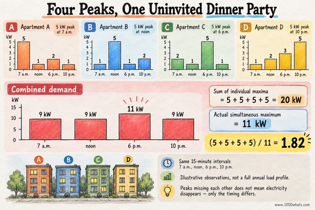
Imagine four neighbors, each with a maximum measured electricity demand of 5 kilowatts (kW). That is not the rating of every appliance they own. It is the highest demand each household actually reaches during the period we are studying.
Neighbor A reaches 5 kW at 7 a.m. while making breakfast. B reaches 5 kW at noon. C peaks at 6 p.m. D peaks at 10 p.m. Individually, they have each hit 5 kW. Collectively, they have never held a meeting about it.
Add their individual peaks and you get 20 kW. But suppose the highest demand measured at the shared connection is only 11 kW. The transformer does not have to supply 20 kW just because the arithmetic department says four times five equals twenty. It has to supply what the four households demand at the same time.
This is the central trick: a collection of loads can have a lower maximum demand than the sum of its members’ individual maximum demands. The difference is not missing electricity. It is missing simultaneity.
What is diversity factor?
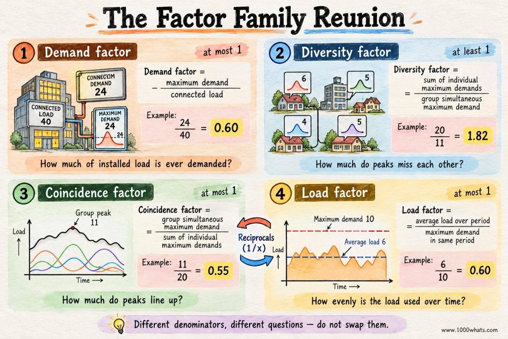
Diversity factor is the sum of the individual maximum demands of a group of loads divided by the maximum demand of that group measured together, over a defined period.
Diversity factor = Sum of individual maximum demands ÷ Maximum simultaneous demand of the group
For our four neighbors: 20 kW ÷ 11 kW = 1.82, rounded. The factor has no units because kilowatts cancel. A value of 1 means every individual maximum can occur together. A value above 1 tells us the peaks do not fully coincide.
Under this definition, diversity factor cannot be less than 1 for a consistently defined group and observation period. The group’s peak cannot exceed the sum of the individual peaks. If your calculation says 0.7, check which way you divided. The laws of mathematics have not filed for an exception.
The formal distinction is also used in Schneider Electric’s distribution design guidance. It separates individual maximum demand from the maximum demand of the combined system, which is precisely the distinction our imaginary neighbors are busy demonstrating.
Four neighbors, one transformer, and a spreadsheet with good news
Let us give the neighborhood actual readings. All values below are illustrative average powers over the same 15-minute intervals. The table is not a universal residential load profile, just a transparent example.
| Time | A (kW) | B (kW) | C (kW) | D (kW) | Combined (kW) |
|---|---|---|---|---|---|
| 7 a.m. | 5 | 2 | 1 | 1 | 9 |
| Noon | 1 | 5 | 2 | 1 | 9 |
| 6 p.m. | 2 | 3 | 5 | 1 | 11 |
| 10 p.m. | 1 | 1 | 2 | 5 | 9 |
Each household reaches 5 kW in one of these intervals. Add the individual maxima and you get 20 kW. The largest combined value in the table is 11 kW, at 6 p.m. Therefore the diversity factor for this illustrative four-interval dataset is 20/11, or about 1.82.
Notice the trap: we are not adding the 7 a.m. peak of A to the noon peak of B and pretending that both happened at 6 p.m. That would be like billing a restaurant for every customer who has ever occupied a chair, all at once. Very profitable. Also, very wrong.
For real engineering, we would examine a sufficiently representative measurement period, with suitable time resolution, rather than four convenient snapshots. But the arithmetic remains the same.
Coincidence factor: the same party viewed from the other side
Electrical engineering has a second number that looks at the same situation from the opposite direction. Coincidence factor is the maximum simultaneous demand of the group divided by the sum of the individual maximum demands.
Coincidence factor = Group maximum demand ÷ Sum of individual maximum demands
For our neighbors, that is 11/20 = 0.55, or 55%. The diversity factor is its reciprocal: 1/0.55 ≈ 1.82.
The coincidence factor asks, “What fraction of everyone’s separate peaks turned up together?” The diversity factor asks, “How much larger is the sum of those separate peaks than the group peak?” Same dinner party. Different seating chart.
Here is a terminology warning worth keeping: some design guides use the word diversity informally for a factor below 1, when they are really applying a coincidence or simultaneity factor. The Electrical Installation Guide explicitly flags this naming confusion. Never trust the label alone. Check the formula before multiplying or dividing anything expensive.
Demand factor, load factor, diversity factor: three relatives who are not twins
A building engineer can spend an entire afternoon in a meeting where everybody says “factor” and nobody means the same one. Let us rescue that afternoon.
| Measure | Formula | Question it answers |
|---|---|---|
| Demand factor | Maximum demand ÷ Connected load | How much of the installed equipment rating is demanded at the peak? |
| Diversity factor | Sum of individual maxima ÷ Group maximum | How much do individual peaks fail to overlap? |
| Coincidence factor | Group maximum ÷ Sum of individual maxima | How much of those individual peaks occurs together? |
| Load factor | Average demand ÷ Maximum demand | How steadily is the load used over time? |
Suppose a workshop has 100 kW of connected equipment but its maximum measured demand is 60 kW. Its demand factor is 0.60. That tells us the workshop does not demand its entire connected rating at once. It does not tell us how its peak lines up with the neighboring workshop’s peak.
Suppose a feeder averages 30 kW over a month and reaches a 60 kW maximum during that same month. Its load factor is 0.50. That describes the shape of its own demand over time. It does not tell us how many separate customers have different peak hours.
And suppose two workshops each peak at 60 kW, while their combined feeder peaks at 90 kW. Their diversity factor is 120/90 = 1.33. Now we are talking about the timing relationship between loads. Three questions, three answers, three opportunities to avoid sizing a cable using the wrong number.
Why diversity saves real money
Power networks are built for demanding moments, not just for annual energy totals. Transformers, cables, switchgear and other equipment must handle expected peak loading within their electrical and thermal limits. They also need appropriate margins for growth, contingencies and applicable design standards.
Imagine a group of customers whose individual maximum demands add up to 1,000 kW. If credible measurements and planning assumptions support a diversity factor of 1.25, the group’s estimated maximum coincident demand is 1,000/1.25 = 800 kW.
That does not mean an 800 kW transformer is automatically the right purchase. Transformers are commonly rated in kVA, not kW; power factor matters. Ambient conditions, permissible overloads, protection, voltage drop, reliability criteria and future growth also matter. But it does mean that assuming 1,000 kW of simultaneous demand may exaggerate the actual peak.
Oversize everything and customers pay for steel, copper and capacity they rarely use. Undersize it and a hot evening can turn your carefully optimized network into a demonstration of the phrase “thermal limit.” Diversity is how planners try to avoid both mistakes.
There is a subtle point here. Diversity does not reduce the energy that customers consume simply by existing. Four households can consume the same total kilowatt-hours while spreading their use across different hours. Diversity primarily changes the combined peak power requirement, not the arithmetic of the electricity bill’s energy component.
The 100-household mistake
Now scale up the apartment building. Suppose 100 homes each have a 10 kW individual maximum demand over a suitable period. Their separate maxima sum to 1,000 kW. It would be reckless to declare that the neighborhood therefore needs 1 MW of simultaneous capacity. It would be equally reckless to announce that it needs exactly 300 kW because somebody once saw that number in a slide deck.
The real coincident peak depends on the households, weather, appliances, heating and cooling systems, electric vehicles, local habits and the observation period. Residential diversity is not a magic discount coupon with a universal percentage printed on the back.
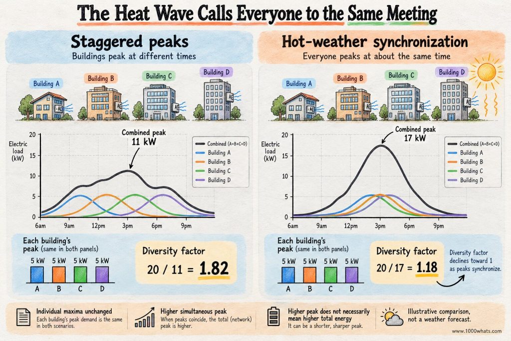
Large populations often exhibit useful averaging because not everybody behaves identically. But their common influences can also make them move together. The first freezing evening of winter can convince thousands of heat pumps to join the same meeting. A heat wave can do something similar with air conditioners.
The lesson is wonderfully inconvenient: people are different until the weather gives them a common agenda.
The electric car arrives and rearranges the seating plan
An EV charger is not automatically a problem for diversity. It is another load with a power level and a schedule. The schedule is the interesting part.
If many drivers plug in after work and immediately charge at high power, their charging demand may overlap with cooking, heating and other evening loads. The neighborhood’s combined peak can rise. But if charging is spread across the night or managed in response to local constraints, the same amount of charging energy may create a much smaller additional peak.
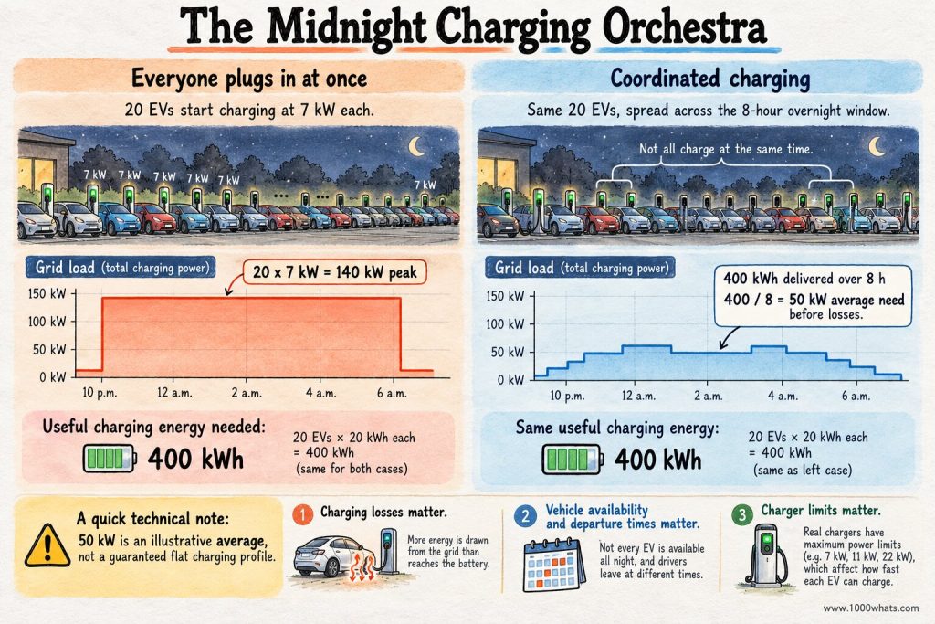
Take 20 vehicles, each needing 20 kWh overnight. Together they need 400 kWh. If every vehicle charges at 7 kW at once, the charging component alone reaches 140 kW while all 20 are active. If their charging is coordinated evenly across an eight-hour window, the average charging power needed is 400/8 = 50 kW, before losses. Actual charging schedules must respect charger ratings, battery requirements, departure times and network constraints, but the difference between 140 kW and roughly 50 kW explains the opportunity.
This is where demand response and smart charging become more than fashionable phrases. They can change when electricity is used, not necessarily how much useful service people receive.
A caution: do not interpret 50 kW as a guaranteed achievable constant grid draw. Charging losses increase the energy required at the plug, and real schedules are constrained. The example isolates the timing principle, not a finished control design.
The coincidence nobody wants: synchronized peaks
Diversity has a natural enemy: synchronization. Picture an office district with many similar buildings. Their air-conditioning peaks may cluster in the afternoon. Picture a residential neighborhood where electric heating, cooking and vehicle charging all rise on a cold evening. Picture a factory campus where every production line starts at the same shift change.
When previously separate peaks become more aligned, coincidence factor rises and diversity factor falls toward 1. The same collection of customers can impose a larger group peak without every customer increasing their individual maximum.
This is why historical diversity factors deserve respect, not worship. A neighborhood measured before widespread electrification may not behave the same way after hundreds of heat pumps and EV chargers arrive. Yesterday’s load shape is useful evidence, but it is not a lifetime warranty.
And yes, rooftop solar complicates the story further. Midday photovoltaic output may reduce net demand at some connections, while evening demand remains high. Depending on how load and generation are metered and defined, net-load peaks can shift. A diversity study must say whether it is examining gross consumption, net imports, or another clearly defined quantity. Otherwise we may be comparing apples, oranges and a solar inverter.
Does a higher diversity factor always mean a better grid?
A higher factor can indicate that individual maxima are less coincident, which can reduce the group’s peak relative to their sum. But it is not a universal quality score. It can change because of customer mix, measurement period, weather, data granularity or how loads are grouped.
A diversity factor of 2 for one feeder does not automatically make it cheaper or more reliable than another feeder with a factor of 1.4. The first might have twice the customers, a longer cable, poor voltage conditions or a very different risk profile. The number answers a narrow but valuable question. Do not promote it to chief executive of the entire grid.
Likewise, diversity is not a substitute for engineering standards. Some circuits serve safety-critical or highly correlated loads. Some require firm capacity for foreseeable simultaneous operation. Others may rely on verified controls that limit coincident demand. The appropriate assumption follows the duty, not the engineer’s appetite for a smaller transformer.
How utilities actually use it
Utilities and electrical designers estimate coincident peaks from measurements, customer classes, load research, models and planning rules. In some contexts they use after diversity maximum demand (ADMD), a related planning metric that expresses the group peak per customer once diversity is taken into account.
If 100 similar homes have a combined measured maximum of 400 kW, their ADMD is 400/100 = 4 kW per home for that particular group, period and definition. It does not mean each home is limited to 4 kW. One may briefly demand 9 kW while another is using 1 kW. ADMD describes the group, averaged per connection.
Do not confuse it with an individual household’s maximum or a universal constant that can be copied between climates. For a new development, planners may need to account for customer composition, local heating fuel, EV uptake, future growth and uncertainty.
The Engineering Institute of Technology discusses ADMD alongside diversity in distribution planning. It is a reminder that the engineering objective is not to guess what every home might do in isolation, but to estimate what the network will actually have to carry together.
How to calculate diversity factor without fooling yourself
The arithmetic is short. The data discipline is not. First, define the exact group of loads and the measurement period. Second, measure each member’s maximum demand over that period using a consistent demand interval. Third, sum those individual maxima. Fourth, measure the maximum of the combined demand over the same period and interval. Finally, divide.
That consistency matters. Comparing one customer’s one-second instantaneous spike with another customer’s 15-minute average, then dividing by a feeder’s hourly average, produces a number with impressive decimal places and very little meaning.
There is also a boundary problem. If your customer meters record imports while a feeder meter includes local generation, losses or unmetered loads, the two sides of the ratio may not describe the same system. Define the electrical boundary, treatment of exports and losses, and whether you are using kW, kVA or current. A ratio of unlike quantities is not diversity. It is bookkeeping cosplay.
And remember that a diversity factor calculated from past observations is descriptive. Turning it into a forecast requires a defensible view of future behavior. You cannot forecast tomorrow’s orchestra by measuring only yesterday’s soloists.
A final thought about the people behind the power curve
There is something quietly delightful about this concept. We spend much of modern life trying to synchronize everything: calendars, trains, deliveries, devices, meetings. The electricity grid often benefits from the opposite. The person who cooks early, the person who works late and the person who charges a car after midnight are doing the network a favor without ever signing a cooperation agreement.
That favor has limits. Shared weather, shared habits and new technologies can bring the peaks together. Smart controls can help spread them apart again. Diversity is not a free source of energy. It is the practical value of not needing all the power at once.
Final thoughts
Diversity factor compares the sum of individual maximum demands with the maximum demand of the group. It explains why separate peaks cannot simply be added to size a shared network, and why the timing of electricity use can be as important as the amount.
The next time somebody tells you that a hundred homes each need 10 kW, so their transformer must serve 1,000 kW simultaneously, ask one question: Did all those peaks RSVP for the same hour?
Until next time, stay curious! 😎
Discover more from 1000whats
Subscribe to get the latest posts sent to your email.