
At 12:07 p.m., a solar farm is having the best day of its life. The sky is spotless. The panels are humming. Somewhere in the control room, a spreadsheet is beginning to feel attractive. Then the inverter announces that it is full.
Not broken. Not overheated. Not on strike. Just full. The panels could offer more power, but the machine that turns their direct current into grid-ready alternating current has reached its limit. It is the electrical equivalent of a restaurant with forty hungry customers and a kitchen that can cook thirty dinners an hour. The chef is excellent. The queue is not his problem.
This is solar inverter clipping. It sounds like an unfortunate haircut, but it is often an intentional design decision. The surprising part is that a solar project can deliberately leave some sunny-hour energy unharvested and still produce more electricity over the year, at a lower cost.
Welcome to 1000whats, where today we are going to ask a slightly impolite question: Why would anyone install more solar panels than their inverter can handle?
First, meet the two nameplates that refuse to agree
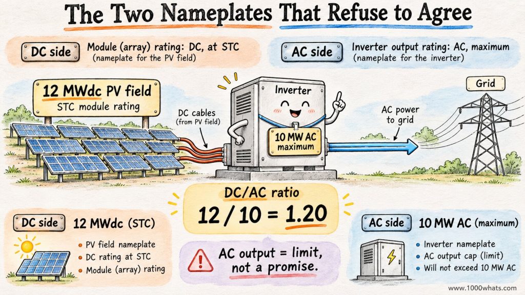
Solar panels produce DC electricity. An inverter converts it to AC electricity that can serve loads or enter the grid. Both sides have power ratings, but they are not the same kind of rating. A 10 MWDC solar array is not automatically a 10 MWAC generating plant. Treating the two as interchangeable is how perfectly respectable project meetings become interpretive theater. The DC and AC ratings are colleagues who share an office but refuse to share a business card. One measures what the solar array can offer under reference conditions; the other measures what the inverter can actually send out. Ask them for a single number and both will confidently point at the other.
The array’s DC nameplate is generally based on standard test conditions, including irradiance of 1,000 W/m² and a cell temperature of 25°C. Those are laboratory reference conditions, not a promise that your roof will recreate a pleasant spring afternoon inside a testing chamber every day. Actual module output responds to irradiance, temperature, angle, shading, soiling, and electrical losses. Standard test conditions are the solar industry’s version of a professional headshot: excellent lighting, flattering temperature, and absolutely no guarantee that Tuesday will look like that.
The inverter’s AC rating describes the maximum AC power it can continuously deliver under its specified conditions. Its conversion efficiency is less than 100%, and its actual capability may depend on temperature, voltage, reactive-power obligations, and equipment settings. For our worked examples, we will use a simplified, constant 96% conversion efficiency and clearly mark where real engineering needs more detail. A real inverter is not a bottomless electrical buffet. Even if the modules arrive carrying enough DC power to feed a small parade, its AC rating still gets the final say.
DC/AC ratio = installed DC nameplate capacity ÷ inverter AC nameplate capacity. It is also called the inverter loading ratio, or ILR. The order matters. A 12 MWDC array feeding a 10 MWAC inverter has a DC/AC ratio of 1.20, not 0.83. Inverting the fraction does not make the inverter bigger. It just makes the spreadsheet less helpful.
| Item | Example rating | What it describes |
|---|---|---|
| Solar modules | 12 MWdc | Array output under reference conditions |
| Inverter | 10 MWac | Maximum continuous AC output under rated conditions |
| DC/AC ratio | 12 ÷ 10 = 1.20 | Installed DC nameplate relative to AC rating |
Ratios above one are common because panels rarely operate at their full DC nameplate for long. A larger array helps fill the inverter’s available capacity on weaker-sunlight hours. The trade-off is that, on particularly productive hours, the inverter reaches its ceiling and cannot convert every additional potential watt. This is not a universal recipe: the best ratio depends on weather, equipment, financing, grid limits, and the value of electricity at different hours. Think of the extra panels as hiring more breakfast staff for a restaurant whose lunch kitchen has a fixed number of burners. You may occasionally turn customers away at noon, but you stop serving an empty dining room at 9 a.m. The economics are in the whole day, not the chef’s most dramatic five minutes.
What clipping actually does, without inventing a tiny electrical bonfire
An inverter does not normally accept unlimited extra DC energy and then heroically burn it off as heat. Its controls change the operating point of the photovoltaic array, so the panels deliver less than their available maximum-power-point output. In plain English, the inverter declines to collect some potential energy. It is a bouncer with excellent semiconductor manners. The panels are not being secretly interrogated in a room full of resistors. Their operating point is adjusted, so some of the sunlight that could have become electricity simply does not become electrical output. The sun receives no refund request.
A useful simplified model is potential AC power = available DC power × inverter efficiency. Actual AC output is the smaller of that potential and the inverter’s AC limit. The difference is the clipping loss expressed on the AC-equivalent side. If the array could provide 11 MW DC and efficiency is 96%, potential AC output would be 10.56 MW. A 10 MW inverter delivers 10 MW. The remaining 0.56 MW is unharvested potential AC power during that interval.
That last sentence is deliberately precise. We did not say 1 MW was lost merely because 11 is greater than 10. We accounted for conversion losses first. We also did not say the inverter dumped 0.56 MW into its heat sink. That would turn the control cabinet into a very expensive toaster.
| Available DC | Potential AC at 96% | 10 MW AC ceiling | Clipped AC-equivalent power |
|---|---|---|---|
| 7.0 MW | 6.72 MW | 10.00 MW | 0.00 MW |
| 9.0 MW | 8.64 MW | 10.00 MW | 0.00 MW |
| 10.0 MW | 9.60 MW | 10.00 MW | 0.00 MW |
| 11.0 MW | 10.56 MW | 10.00 MW | 0.56 MW |
| 12.0 MW | 11.52 MW | 10.00 MW | 1.52 MW |
Clipping is a power limit at an instant. To calculate energy lost, we need to know how long that limit persists. This is where the sun, annoyingly, insists on moving across the sky instead of holding still for our convenience. A megawatt is a rate, not a suitcase of energy. Saying “we lost 0.56 MW” without saying for how long is like announcing that a bathtub fills at 20 liters per minute and then refusing to say whether the tap was open during a commercial break or an entire opera.
A six-hour solar day walks into an inverter
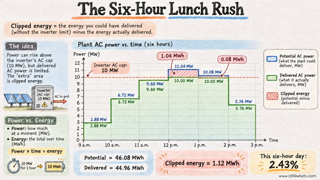
Let us build a tiny solar day with six one-hour intervals. Our array is rated at 12 MW DC, our inverter at 10 MW AC, and conversion efficiency is assumed to be 96% at every interval. The available DC figures are hypothetical, not a measured production profile. They are chosen so that you can audit the arithmetic with a pencil and an attitude.
| Hour | Available DC (MW) | Potential AC (MW) | Actual AC (MW) | Clipped energy (MWh) |
|---|---|---|---|---|
| 9–10 | 3.0 | 2.88 | 2.88 | 0.00 |
| 10–11 | 7.0 | 6.72 | 6.72 | 0.00 |
| 11–12 | 10.0 | 9.60 | 9.60 | 0.00 |
| 12–1 | 11.5 | 11.04 | 10.00 | 1.04 |
| 1–2 | 10.5 | 10.08 | 10.00 | 0.08 |
| 2–3 | 6.0 | 5.76 | 5.76 | 0.00 |
| TOTAL | 48.0 MWh DC | 46.08 MWh AC-equivalent | 44.96 MWh AC | 1.12 MWh |
The two clipping hours lose 1.04 + 0.08 = 1.12 MWh of potential AC output. Without the AC ceiling, the simplified conversion model would produce 46.08 MWh. With it, we deliver 44.96 MWh. So the clipping fraction of potential AC energy for this six-hour example is 1.12 ÷ 46.08 = 2.43%. That is not an annual clipping estimate. It is the result for these six invented hours. A day is not a year, even if your Monday occasionally feels like one. In the control room, the production graph has acquired a very tidy haircut. The finance team calls the flat top a loss. The engineer calls it a design choice. Both are right, which is why their meetings tend to need coffee.
Notice the shape: output rises, reaches a flat 10 MW plateau, then falls. A power-versus-time chart shows the missing energy as the area between the unconstrained potential-AC curve and the 10 MW line. For one-hour intervals, megawatts multiplied by one hour become megawatt-hours. The units do not negotiate.
A further subtlety: these are hourly average powers. Real clipping can begin and end inside an hour. If you model it using coarse hourly averages, you may miss short peaks. Serious project analysis uses suitable weather and time-resolution data, equipment curves, and uncertainty ranges. Our table is a teaching model, not a substitute for a bankable yield assessment. The sun does not promise to hold still for an hourly spreadsheet. Passing clouds can make the power trace jump around like a cat discovering a laser pointer. Subhourly data can reveal clipping hidden by an innocent-looking hourly average.
The paradox: a bigger array can lose more and deliver more
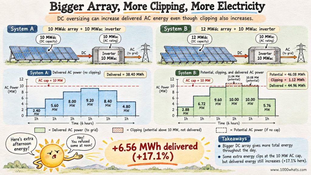
Now imagine two versions of the same site. Both connect through a 10 MW AC inverter. Plant A has 10 MW DC of modules. Plant B has 12 MW DC. They face the same six sunlight intervals, and we assume Plant B’s available DC power is exactly 20% higher at each interval. That scaling is a simplification: in reality, string layouts, shading, temperature, and electrical design complicate matters.
Plant B’s available DC sequence is the one in our previous table: 3, 7, 10, 11.5, 10.5, and 6 MW. Plant A therefore has 2.50, 5.83, 8.33, 9.58, 8.75, and 5.00 MW DC, respectively. At 96% conversion efficiency, Plant A never reaches the 10 MW AC ceiling. It delivers 38.40 MWh. Plant B delivers 44.96 MWh after clipping.
| Metric | Plant A: 10 MWdc / 10 MWac | Plant B: 12 MWdc / 10 MWac |
|---|---|---|
| DC/AC ratio | 1.00 | 1.20 |
| Potential AC energy | 38.40 MWh | 46.08 MWh |
| Clipped energy | 0.00 MWh | 1.12 MWh |
| Delivered AC energy | 38.40 MWh | 44.96 MWh |
| Gain over Plant A | Baseline | 6.56 MWh (+17.1%) |
Plant B sacrifices 1.12 MWh of its own potential output and still delivers 6.56 MWh more than Plant A. It is the only dinner party where throwing away some appetizers can help feed more guests. The reason is not magic: extra modules produce extra energy during the many hours when the inverter is not full. Plant B is the guest who leaves some food on the plate and still eats a bigger dinner. That sounds impossible only if you confuse the percentage eaten with the amount eaten.
This is the essential design trade-off. You are not trying to maximize the percentage of sunlight harvested at every instant. You are trying to optimize the energy, value, and cost of the entire system over its operating life. Those are different objectives. If a contractor says “zero clipping” as though it were a sacred engineering commandment, ask what the system costs and how many kilowatt-hours it delivers.
Now the finance director enters, carrying a calculator and absolutely no joy
Extra modules are not free. Neither are larger inverters, additional cabling, switchgear, maintenance, land, or transformer capacity. The engineering choice becomes an economic question: What is the value of extra delivered energy, and what does the equipment needed to capture it cost? The finance director has now entered the room. He is immune to metaphors, deeply suspicious of sunshine, and has just asked the inverter whether it can produce a discounted cash flow statement.
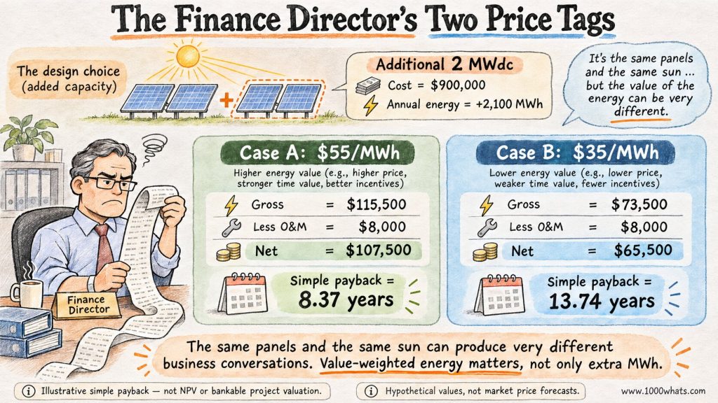
Suppose the extra 2 MW DC of modules costs $900,000 installed, all-in for this incremental comparison. Suppose a site-specific annual simulation, not our six-hour classroom day, predicts 2,100 additional MWh per year after clipping. At an illustrative realized value of $55/MWh, gross incremental annual revenue is 2,100 × $55 = $115,500. If incremental annual operating expense is $8,000, the simplified annual contribution is $107,500.
The simple payback is $900,000 ÷ $107,500 = 8.37 years. This is not a project valuation. It ignores financing, taxes, degradation, inflation, replacement costs, curtailment, merchant-price risk, and the time value of money. The finance director, having briefly smiled, has found eleven new tabs for the spreadsheet.
| Illustrative input | Value |
|---|---|
| Additional installed DC | 2 MWdc |
| Incremental installed cost | $900,000 |
| Extra annual delivered AC energy | 2,100 MWh |
| Realized value | $55/MWh |
| Incremental annual operating cost | $8,000 |
| Annual net contribution | $107,500 |
| Simple payback | 8.37 years |
What if the extra energy is mostly produced at midday, when solar generation depresses wholesale prices? Then $55/MWh may be too generous. If its actual realized value is only $35/MWh, annual gross revenue falls to $73,500 and net contribution to $65,500. Simple payback stretches to 13.74 years. Same panels. Same sun. Very different board meeting. The midday megawatt-hour is not necessarily the glamorous megawatt-hour. If every solar farm arrives at the market simultaneously, the price may behave like a beach hotel trying to sell rooms during a hurricane warning.
A proper comparison uses hourly production and hourly economic value, along with the project’s contractual arrangements. The market does not owe every megawatt-hour the same price. It also does not care that your spreadsheet cell is green.
Why not simply buy a bigger inverter?
Excellent question. We can also keep the 12 MW DC array and increase inverter capacity from 10 MW AC to, say, 12 MW AC. In our simplified six-hour example, this removes all 1.12 MWh of clipping and raises delivered energy from 44.96 to 46.08 MWh. But whether that additional energy justifies the larger inverter is a separate calculation.
Suppose the larger inverter and associated balance-of-system changes cost $250,000 more. Suppose an annual model predicts that the upgrade captures 350 additional MWh a year, valued at $45/MWh, with $2,000 additional annual operating costs. The simplified annual net contribution is 350 × $45 − $2,000 = $13,750. Simple payback is 18.18 years. Again, hypothetical numbers, not an equipment quote.
But change the weather, the project layout, or the value of midday energy, and the result changes. Sometimes a bigger inverter is the sensible choice. Sometimes the extra panels are. Sometimes the connection agreement limits AC export so firmly that a bigger inverter would merely become an expensive monument to optimism. There is no universal magic ratio, despite the confidence with which some slide decks pronounce one. A ratio is a design variable, not a lucky number printed inside a fortune cookie.
And beware the phrase “the inverter is only 10 MW.” Its nameplate may not be the final grid export limit. Transformers, plant auxiliary consumption, reactive-power requirements, grid-connection rules, and control settings can create additional constraints. A 10 MW AC inverter does not promise exactly 10 MW at the point of interconnection every sunny hour.
Clipping versus curtailment: two different ways to hear “not today”
Clipping and curtailment can create similar-looking flat tops in production charts, but they have different causes. Clipping occurs because the conversion equipment reaches an internal capability limit. Curtailment occurs when generation is intentionally reduced because of an external instruction, grid constraint, economic dispatch decision, or contractual limit. Clipping is usually the plant saying, “My equipment has reached its limit.” Curtailment is someone else, or another plant-level constraint, saying, “Please do not send that much.” The graph may look similar, but the responsible parties would prefer you not mix up their names at the meeting.
Imagine our 10 MW inverter is capable of producing 10 MW at noon, but the grid operator requires the plant to export no more than 7 MW for an hour. The plant may produce only 7 MW AC even though its inverter could deliver more. That 3 MW gap is not inverter clipping. It is a dispatch or export restriction. Calling everything clipping is like calling every canceled flight “bad weather.” Sometimes the weather is innocent and the airline has misplaced an aircraft.
A production plateau is therefore a clue, not a diagnosis. To identify the cause, inspect irradiance, available DC power, inverter operating status, plant controller setpoints, reactive-power behavior, and point-of-interconnection measurements. The graph is the witness. It is not the judge.
Temperature, orientation, and the curious case of the noon peak
PV modules generally deliver less power as cell temperature rises, all else equal. So a blazing hot afternoon can produce less DC power than a cooler, clear day with comparable irradiance. Solar panels enjoy sunshine. They are less enthusiastic about being cooked. This matters for clipping because the largest peaks may occur under cool, bright conditions, not simply on the hottest day. Hot solar panels are another of nature’s less intuitive jokes: the sun gives with one hand and heats the semiconductor with the other. Brightness and cell temperature are not the same variable, and the panel has opinions about both.
East-west arrays can spread output over more of the day and lower the noon peak compared with a similarly rated south-facing array, depending on latitude, tilt, and other design choices. Trackers change the shape again. Bifacial modules can add rear-side irradiance. Soiling and shading remove available power. Each changes the hours when the inverter hits its limit.
This is why a single “normal clipping percentage” is dangerous. A ratio of 1.30 can behave differently in two locations, or even on two rooftops across the street with different orientations. The ratio is an input to analysis, not the result of analysis. Anyone who guarantees your annual clipping loss from the ratio alone has either discovered a new branch of meteorology or skipped a few steps.
Can a battery rescue clipped solar energy?
Sometimes. In a suitably designed DC-coupled solar-plus-storage system, a battery converter may be able to charge from DC energy that would otherwise be unavailable to the AC inverter. That can turn some clipping potential into stored energy for later delivery. But it depends on the architecture, battery charge limits, state of charge, control strategy, and electrical ratings. A battery is not a magical bucket placed under the inverter to catch spare electrons. A battery may offer the surplus power a side door, but only if the electrical architecture actually includes that door. Drawing a battery beside a solar farm on a PowerPoint slide does not install the necessary converters, controls, or wiring.
An AC-coupled battery connected downstream of an already saturated solar inverter cannot automatically recover DC power that the inverter never converted. It may absorb available AC output and change export behavior, but the architecture matters. Claims about “capturing all clipped energy” deserve an actual one-line diagram and a simulation, not a stock photo of a smiling battery.
Storage also has round-trip losses and costs. If 1 MWh of previously clipped DC energy becomes 0.85 MWh of delivered AC electricity after conversion and storage losses, it can still be worthwhile if later electricity is sufficiently valuable. But the comparison must use delivered energy, not wishful thinking measured in megawatt-hours.
A few questions worth asking before signing the solar proposal
When someone presents a proposed solar plant, ask for the DC array rating, AC inverter rating, and DC/AC ratio in the same table. Then ask for expected annual AC energy at the point that matters commercially, the modeled clipping loss, and the weather dataset and time resolution used. Request an explanation of any export or curtailment limits, and confirm that the selected inverter can safely accept the planned string voltages, currents, and DC oversizing under the manufacturer’s rules. If the proposal shows one heroic annual MWh number but refuses to show hourly clipping, treat it like a restaurant menu that lists only “food: excellent.” You have learned something about the marketing department, not the meal.
Also ask for a comparison with at least one alternative configuration. A 10 MW AC inverter with 12 MW DC modules may be excellent. It may also be wrong for a particular site. The only respectable answer is one supported by the physical design and the economics. The rest is a sales pitch wearing a hard hat.
Final thoughts
Solar inverter clipping is what happens when the available photovoltaic power could produce more AC electricity than the inverter is able or permitted to deliver. Some potential output goes unharvested during those intervals. It is a real loss, but it is not necessarily a design failure.
The bigger lesson is that optimizing a power plant is not the same as eliminating every visible loss. Extra solar panels can deliver more morning and afternoon energy, even when the noon peak gets its head trimmed. A larger inverter can recover that peak, but only at a cost. The winning design depends on the full year, the full price curve, and the full equipment bill. The engineering question is not “How do we make every loss disappear?” It is “Which combination of equipment, production profile, and market value leaves us with the best outcome?” The first question produces an immaculate graph. The second might produce a profitable power plant.
Our imaginary inverter is still standing at the door, checking IDs. The sun has plenty of energy. The inverter has a capacity limit. The engineer has a spreadsheet. And the finance director has just asked whether the spreadsheet includes degradation.
Until next time, stay curious! 😎
Discover more from 1000whats
Subscribe to get the latest posts sent to your email.