
The calendar had a good job at the electric utility. It knew which Tuesday came after which Monday. It remembered Christmas, heat waves, the occasional national holiday, and the precise hour when everyone returned home and turned on something expensive.
Then an engineer walked into a meeting with 8,760 numbers, rearranged them from biggest to smallest, and announced, “I’ve improved the year.”
January was furious. August found itself sitting next to February. Wednesday had been separated from its family. The calendar asked whether anyone had considered the consequences.
“Of course,” said the engineer. “Look how much easier the graph is to read.”
And, irritatingly, the engineer had a point.
Welcome to 1000whats, where today’s guest is the load duration curve, a remarkably useful electricity-planning tool that takes an entire year of demand and sorts it by size instead of date. It tells you how often the power system was very busy, how much energy it needed, and how much of its capacity spent most of the year waiting for a phone call.
It also has one spectacular weakness: once you fire the calendar, you can no longer tell what happened before or after anything else. We will eventually have to give the calendar its job back. The battery department has already filed a complaint.
First, meet the ordinary load curve
Electricity demand refuses to sit still. At 6 a.m., people wake up. Offices open. Factories change shifts. Air conditioners respond to weather with the subtlety of an orchestra warming up in a broom closet. At night, some loads disappear while others, such as data centers and industrial processes, carry on.
A chronological load curve, often called a load profile, plots that demand against actual time. The horizontal axis might show hours of a day or dates across a year. The vertical axis shows electrical power, usually in kilowatts (kW), megawatts (MW), or gigawatts (GW).
That is a power measurement, not an energy measurement. If demand is 40 MW for one hour, the energy consumed in that hour is 40 MWh. If it is 40 MW for two hours, the energy is 80 MWh. The difference between MW and MWh is the difference between the speedometer and the distance traveled. Confusing them is an excellent way to make an energy engineer stare silently at the ceiling.
The chronological graph is essential for operations. It tells the dispatcher when the morning rise begins, whether the evening peak is getting steeper, and whether tomorrow’s maintenance outage overlaps with a difficult hour. In short, it respects the calendar. For a closer look at keeping supply and demand together in real time, see my explanation of electricity balancing.
But suppose the question is different: For how many hours did demand exceed 30 MW? A chronological graph makes you hunt through the year, adding little intervals as if collecting receipts after a particularly irresponsible vacation.
The load duration curve offers a less sentimental method.
The trick: keep every hour, throw away its name tag
Take all the measured demand values for a period. Sort them from highest to lowest. Plot the sorted values against their rank or cumulative duration. That is the entire basic recipe for a load duration curve (LDC).
The tallest hour goes first, even if it happened on a Thursday in July. The quietest hour goes last, even if it occurred the following Tuesday. All the other hours form an orderly descending slope. It is the only meeting at the utility where the highest-maintenance participants are deliberately seated at the front.
Nothing has happened to the measured power values. We have changed only their order. A year with 8,760 hourly readings still contains 8,760 hourly readings, assuming a 365-day year and a consistent hourly time basis. The calendar’s personal feelings are not included in the dataset.
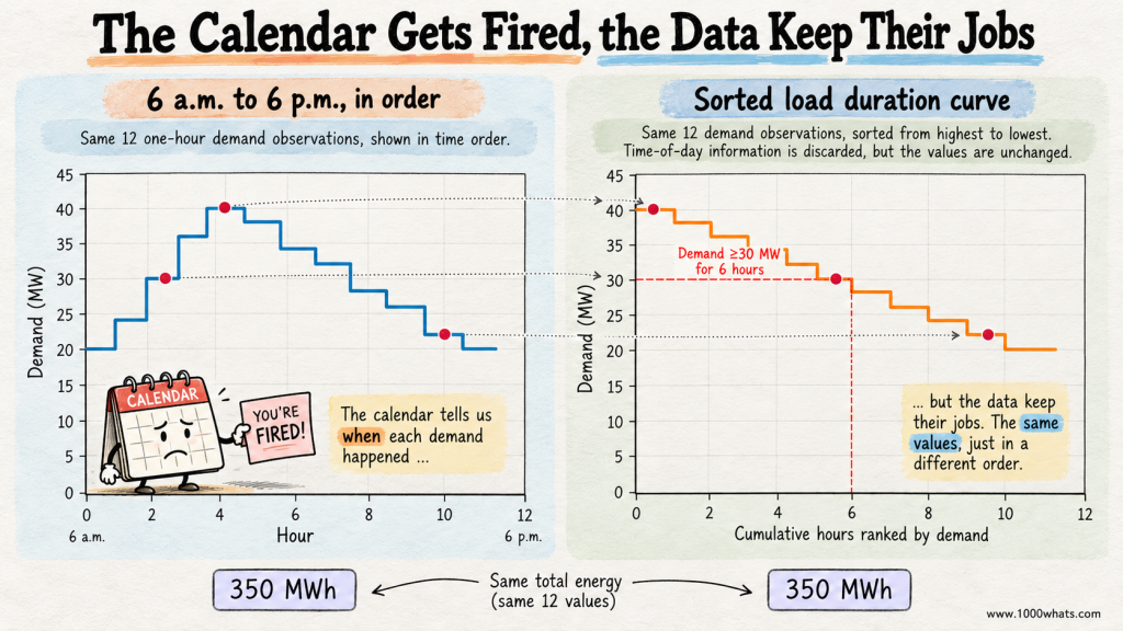
Here is a small example. Imagine a miniature electricity system observed over twelve consecutive one-hour intervals, from 6 a.m. to 6 p.m. The figures are invented to make the arithmetic visible.
| Hour beginning | Actual demand (MW) | Demand after sorting (MW) |
|---|---|---|
| 06:00 | 20 | 40 |
| 07:00 | 24 | 38 |
| 08:00 | 30 | 36 |
| 09:00 | 36 | 34 |
| 10:00 | 40 | 32 |
| 11:00 | 38 | 30 |
| 12:00 | 34 | 28 |
| 13:00 | 32 | 26 |
| 14:00 | 28 | 24 |
| 15:00 | 26 | 22 |
| 16:00 | 22 | 20 |
| 17:00 | 20 | 20 |
The third column is not the demand that actually occurred at the hour shown in the first column. It is the sorted ranking, displayed alongside the chronological series for comparison. At 6 a.m., actual demand was 20 MW, not 40 MW. The first sorted position merely happens to contain the highest reading of the twelve-hour period.
That distinction is the whole game. A chronological load curve answers when? A load duration curve answers how much, for how long?
In our example, demand was at least 30 MW for six hours. It was strictly above 35 MW for three hours. Those answers are immediate once the values are sorted. No calendar excavation required.
How to read the curve without getting tricked by the axes
On the vertical axis is demand in MW. On the horizontal axis is cumulative duration: hours, or sometimes the percentage of the study period. At the far left sits the maximum observed demand. At the far right sits the minimum.
For an annual curve, a point at 1,000 hours and 800 MW can be interpreted, subject to how the steps and ties are plotted, as approximately 1,000 hours with demand at or above 800 MW. If the axis uses percentages, the same idea applies: 10% means roughly the highest-demand tenth of the observed intervals.
The curve never slopes upward as you move right. It cannot. We sorted it that way. If your load duration curve suddenly climbs halfway across, either you have discovered a new branch of mathematics or the spreadsheet is expressing an opinion.
There are three especially useful things to notice.
- The left edge is the peak. It shows the highest measured demand over the chosen interval and period. It does not, by itself, determine all the firm capacity needed for reliability.
- The right edge is the minimum. It reveals how low demand went. That matters when generation has technical minimum-output constraints or when renewable production is abundant.
- The shape tells you how often different demand levels occur. A steep left-hand tip means a small number of unusually demanding hours. A flatter profile means load is more consistent.
Two systems can have the same peak and the same annual energy yet have different load duration curves. One may spend thousands of hours close to its maximum; the other may have a dramatic peak that appears briefly, takes a bow, and leaves the utility with a large bill for capacity it barely uses.
The curve is therefore a portrait of utilization, not just size. A 40 MW peak tells you how tall the building is. The rest of the curve tells you how many floors actually have tenants.
The area under the curve is electricity, not decoration
Now for the feature that makes this chart more than a beautifully organized complaint about busy hours.
The area under a load duration curve equals the total electrical energy represented by the readings. That is because each horizontal slice of time contributes power multiplied by duration. Sorting the slices does not change their sum.
Our twelve hourly values add up to 350 MW when considered simply as numbers. But the physically meaningful energy calculation is:
Energy = sum of hourly power readings × 1 hour = 350 MWh.
We can divide by twelve hours to find the average demand:
Average demand = 350 MWh ÷ 12 h = 29.17 MW.
And we can compare that average with the 40 MW peak:
Load factor = 29.17 MW ÷ 40 MW = 72.9%.
Load factor is a compact description of how steadily demand uses its observed peak capacity. It is not an efficiency rating, and it does not say that 27.1% of electricity was wasted. That would be like accusing a restaurant of wasting chairs whenever the lunch rush ends.
The same calculation works for a year: total MWh divided by the hours in the study period gives average MW; average MW divided by peak MW gives load factor. In a standard 365-day year, that is 8,760 hours. Leap years have 8,784. Analysts must also handle daylight-saving time and missing or duplicated interval records consistently. The grid is not impressed by a dataset with 8,759 hours and an optimistic attitude.
The relationship between power, energy and utilization is also why a load duration curve is not a capacity credit calculation. Capacity credit asks about a resource’s contribution to system reliability. Load factor asks how much demand occurred on average relative to its peak. Same general neighborhood of engineering, very different addresses.
Three layers of demand, and the expensive top floor
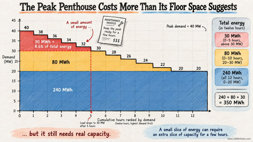
Let’s put our twelve-hour curve to work. Imagine slicing the area beneath it into three horizontal bands: 0–20 MW, 20–30 MW, and 30–40 MW.
The bottom band is present in every one of our twelve hours because demand never falls below 20 MW. The middle band appears when demand rises above 20 MW. The top band is needed only when demand exceeds 30 MW.
Here is the accounting, using the same readings and assuming one-hour intervals.
| Demand band | Energy in twelve hours | What it tells us |
|---|---|---|
| 0–20 MW | 20 MW × 12 h = 240 MWh | A 20 MW demand floor is present throughout. |
| 20–30 MW | 80 MWh | Demand frequently rises above the floor, but not always by the full 10 MW. |
| 30–40 MW | 30 MWh | The highest 10 MW band contributes relatively little energy. |
| Total | 350 MWh | Exactly the same energy as the original time series. |
For the middle band, six intervals contribute the full 10 MW, followed by contributions of 8, 6, 4 and 2 MW: 60 + 8 + 6 + 4 + 2 = 80 MWh. The top band contributes 10 + 8 + 6 + 4 + 2 = 30 MWh. Every MWh has an address. None has been invented by the chart.
This is the classic planning insight. The last 10 MW of peak demand represents 25% of the system’s observed peak power, but only 30 ÷ 350 = 8.6% of its energy over this twelve-hour example.
Imagine owning a piece of equipment that must be available for those upper slices but earns relatively few operating hours. The capital bill arrives every month. The energy sales do not necessarily follow. That is why power systems care about both the cost of installing capacity and the cost of operating it.
Traditionally, planners described the demand stack as baseload, intermediate load, and peak load. Technologies with high fixed costs and low variable costs often made sense at high utilization, while lower-capital-cost, higher-running-cost technologies could be economical for brief peaks. But this is a planning intuition, not a law assigning each colored band to a particular fuel. Actual dispatch depends on renewable output, fuel and carbon prices, flexibility, outages, network constraints, market rules and much more. For the dispatch side of the story, meet the merit order.
The duration curve tells you how much capacity might be used for how long. It does not automatically tell you which generator will run, what it will earn, or whether the power can reach the right place.
The annual version: 8,760 hours, one surprisingly tidy silhouette
Our twelve-hour demonstration is a toy system. A real annual load duration curve can compress an entire year’s hourly demand into a single descending line. On one page, a planner can see how many hours demand exceeded 90% of the annual peak, what the typical load level was, and how much of the year’s energy sat beneath each part of the curve.
Consider two imaginary regions, each with a peak of 10,000 MW.
Region A spends much of the year near 8,000 MW. Region B usually needs only 5,000 MW but occasionally surges to 10,000 MW during extreme weather. The peaks match, but their annual energy needs and utilization patterns can differ dramatically. A planner who sees only “10 GW peak” has received the headline and missed the entire article.
A duration curve can also make energy-efficiency measures easier to discuss. A permanent reduction in a continuously running industrial load changes many hours of the curve. A targeted program that reduces demand on a few very hot afternoons may barely change annual MWh while materially lowering the highest peak. Those are different benefits, and the shape helps separate them.
However, the curve is not a weather forecast, an equipment inventory, or a guarantee that every demand hour can be served. It is a statistical summary of a specified period. If the future contains new electric heating, different industrial shifts, more air conditioning, or thousands of vehicles charging at the same time, yesterday’s tidy silhouette may need an entirely new wardrobe.
Why the tallest hours can be the most expensive hours
The far-left tip of the duration curve deserves a special kind of attention. Suppose a system needs an extra 500 MW for only a handful of hours per year. The equipment, transmission capability, fuel arrangements, and reserves associated with meeting those hours may have costs that are not proportional to the tiny amount of extra energy consumed.
That does not mean every brief peak requires a new gas turbine. It could be addressed by demand response, storage, imports, better network use, flexible generation, or some combination. It also does not mean a peak can be safely ignored because it is rare. Hospitals are grateful that emergency exits are not evaluated solely by how often they are used.
What matters is the distinction between capacity and energy. Capacity is how much power can be supplied at a moment. Energy is how much power is supplied over time. A small area near the top of the curve can still require a large amount of dependable instantaneous capability.
And reliability planning needs more than this graph. A 10,000 MW peak does not imply that exactly 10,000 MW of installed nameplate capacity is sufficient. Generator outages, variable renewable availability, imports, reserves, extreme events and demand uncertainty all matter. Our separate article on capacity credit and ELCC explains why the system cannot simply count every megawatt on a nameplate as a dependable employee.
The load duration curve can show the size and frequency of the mountain. It cannot promise the climbing team will be available on the day of the ascent.
Then solar arrives and changes the guest list
So far, we have sorted gross electricity demand. But the grid increasingly has another important question: how much demand remains for other resources after variable renewable generation has been accounted for?
That remaining requirement is often called net load or residual load. In a simplified hourly calculation:
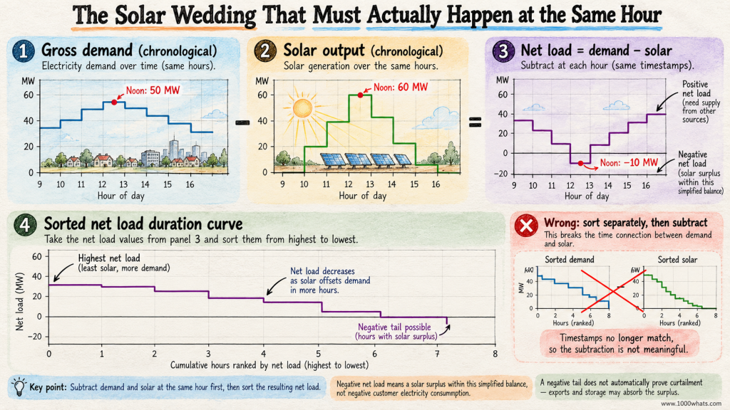
Net load = electricity demand − wind generation − solar generation.
The subtraction must happen hour by hour, before sorting. This detail matters enormously. You cannot sort annual demand, sort annual solar output separately, subtract the two ranked lists and expect to obtain the actual net load duration curve. That would match the sunniest hour with the highest-demand hour whether or not they ever met. A statistical arranged marriage is still an arranged marriage.
For example, suppose demand is 50 MW at noon and solar production is 60 MW. The simplified net load is −10 MW. That does not mean customers are consuming negative electricity. It means local variable generation exceeds the demand included in this simplified balance during that interval. Exports, storage charging, curtailment or other system actions may be needed, depending on the system boundary and constraints.
Sort those correctly calculated hourly net-load values and you have a net load duration curve. Its low end may fall below zero. Its high end shows when dispatchable resources, storage discharge, imports or other flexibility may be most needed. The International Energy Agency’s modeling documentation describes how simplified load-duration segments and residual-load concepts can support power-sector analysis. A National Renewable Energy Laboratory modeling report also distinguishes load, net-load and incremental load-duration curves when examining power-system needs.
Solar can reduce net load substantially at midday while leaving evening demand less affected. That is part of the story behind the duck curve. But the duck curve is chronological: it shows the afternoon dip and evening climb in their proper order. The net load duration curve sorts the same kind of values by magnitude. One shows the choreography; the other shows the cast arranged by height.
With growing renewable generation, that distinction becomes less academic and more operational.
The calendar files an appeal: the curve has forgotten every ramp
Here is the flaw we promised at the beginning. A load duration curve retains the distribution of demand values, but it destroys their sequence.
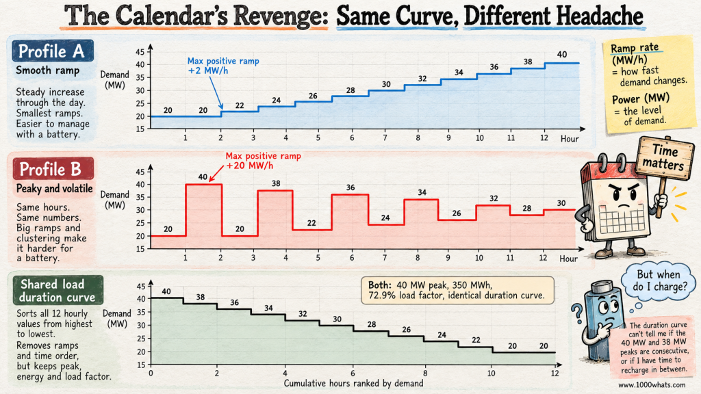
Consider two imaginary twelve-hour demand profiles. Both contain exactly these values: 20, 20, 22, 24, 26, 28, 30, 32, 34, 36, 38 and 40 MW.
In Profile A, demand climbs smoothly: 20, 20, 22, 24, 26, 28, 30, 32, 34, 36, 38, 40.
In Profile B, demand jumps around: 20, 40, 20, 38, 22, 36, 24, 34, 26, 32, 28, 30.
Both have a 40 MW peak. Both use 350 MWh. Both have the same average demand and load factor. Most importantly, both produce exactly the same load duration curve.
But they are not the same operating day. Profile A asks the system to increase output gradually. Profile B repeatedly asks it to change by enormous amounts between adjacent hours. Its biggest one-hour rise is 20 MW; the smoothly rising profile’s biggest is only 2 MW.
That difference matters to ramping resources, storage, balancing arrangements, generator startup decisions and network operations. The duration curve is innocent of any wrongdoing. It simply never promised to remember the order. It is a yearbook, not a surveillance video.
For an explanation of why timing and steep ramps matter when solar production fades, see my article on the duck curve. The calendar, meanwhile, would like an apology in writing.
Batteries insist on knowing what happened yesterday
Storage makes the missing chronology impossible to ignore. A battery has at least two important limits: how quickly it can deliver power, measured in MW, and how much usable energy it can deliver, measured in MWh. It must also have enough charge at the right time.
Return to our original twelve-hour example. The two highest readings were 40 MW and 38 MW, in adjacent one-hour intervals. Suppose we want to cap the system’s demand at 36 MW by discharging a battery during those hours.
At the 40 MW hour, the battery must provide 4 MW for one hour = 4 MWh. At the 38 MW hour, it must provide 2 MW for one hour = 2 MWh. In this simplified calculation, peak shaving therefore requires 4 MW of discharge capability and 6 MWh of usable delivered energy across those two hours.
The load duration curve reveals the 6 MWh area above the 36 MW threshold. Nice. The accountant applauds. The battery operator asks a less glamorous question: “Was I charged before the first hour?”
The duration curve cannot answer. It also cannot tell you whether the peaks were consecutive, whether there was time to recharge between them, or whether the battery was already committed to another service. Our original chronological profile happens to show adjacent peaks, but that information vanished when we sorted it.
Real battery design must also allow for round-trip losses, usable state-of-charge limits, degradation, dispatch uncertainty and the energy required to recharge. A battery delivering 6 MWh generally needs more than 6 MWh of charging electricity over the full cycle. The duration curve cannot negotiate with thermodynamics.
For this reason, duration curves are useful screening tools, but chronological simulation is essential for serious storage scheduling and reliability analysis. This is also why pumped-storage hydropower cannot be sized sensibly from a sorted demand chart alone. Water reservoirs, like batteries, have a memory.
The calendar is now back on the payroll, although management has changed its job title to “temporal integrity specialist.”
Can you flatten the curve without using less electricity?
Absolutely. You can shift electricity consumption from busy hours to quieter ones. Think of charging vehicles overnight instead of at the early-evening peak, or precooling a building before a high-demand period when thermal comfort and operating constraints allow it.
With ideal, lossless shifting, total MWh stays the same but the demand profile changes. The load duration curve may become flatter: lower peaks and somewhat higher low-demand hours. In reality, storage and thermal shifting can introduce losses, so total electricity consumption may rise slightly even while the peak falls.
That is different from reducing electricity use through efficiency. If a lighting retrofit cuts demand during every operating hour, the area under the curve can shrink. If a demand response program merely postpones consumption, the energy may reappear later. If the program truly eliminates consumption, the area can fall.
Three interventions can therefore look superficially similar near the left edge while producing different energy totals, costs, emissions and customer impacts.
| Intervention | Likely effect on peak | Likely effect on total energy | What to check |
|---|---|---|---|
| Permanent efficiency improvement | May reduce it | Usually decreases | Which hours actually change? |
| Load shifting | Can reduce it | Roughly unchanged before losses | Where does the load reappear? |
| Battery peak shaving | Can reduce grid imports at peak | Grid-import energy may increase due to losses | Charge timing, usable MWh and discharge MW |
The key word is may. A household shifting a dishwasher cycle might reduce its own evening peak without affecting the system’s annual maximum at all. For a system-wide benefit, the reduction must occur during the hours that actually drive system needs. This is where my explanation of diversity factor adds another useful piece: the timing of individual peaks determines how they combine.
“Flatten the curve” is not a complete engineering instruction. It is the beginning of a conversation about which curve, whose peak, and when.
Does the load duration curve tell you electricity prices?
No. It is not a price forecast wearing a sensible jacket.
Demand matters to wholesale prices, but prices also depend on available generation, fuel costs, renewable output, imports, network constraints, outages, bidding and market design. Two hours with identical demand can have very different prices if one has abundant wind and the other has a shortage of available generation.
You can construct a price duration curve by sorting hourly electricity prices from highest to lowest. That answers how often a price threshold was exceeded. But, again, it discards the timestamps. It cannot tell you whether high-price hours coincided with your solar output or whether your battery could move energy between low- and high-price periods.
For a generator, the value of electricity depends on when it produces, not simply on how often prices were high. My articles on capture price and energy arbitrage explore that distinction. The sorted-price graph is a useful portrait of the market’s mood swings, but it is not a trading strategy. Buying low and selling high becomes awkward when you have thrown away the appointment book.
How to build a load duration curve without fooling yourself
The arithmetic is simple enough for a spreadsheet. The discipline is in the input data.
- Choose the boundary. Are you measuring a household, a factory, a distribution feeder, or an entire electricity system? Demand measured at a meter is not necessarily the same as total end-use consumption inside that boundary.
- Choose the interval. Hourly, 30-minute and 15-minute readings can produce different observed peaks. A short spike may disappear inside an hourly average.
- Clean the time series. Check missing records, duplicated hours, time zones, daylight-saving transitions and leap years. Keep the energy accounting consistent.
- Sort the demand values from highest to lowest. Do not sort dates and do not sort renewable generation independently before calculating net load.
- Plot power against cumulative duration. Use hours or percentage of intervals, and label the vertical axis with the correct unit.
- Check the area. For equal-length intervals, sum power × interval duration. It must match the original time series’ energy total, within rounding.
- Keep the original chronological data. You will need it for ramping, storage, weather correlations, dispatch, prices and reliability studies. The calendar deserves at least a backup copy.
With unequal interval lengths, do not blindly count each reading as one equal-width hour. Weight observations by their actual durations. With a consistent one-hour series, the standard shortcut works beautifully; with mixed or irregular intervals, careless sorting can give the wrong area.
The U.S. Department of Energy’s energy-efficiency impact evaluation guide uses load duration curves to explain how demand levels relate to the generation mix. The International Energy Agency likewise defines a load or net-load duration curve as a profile sorted by magnitude rather than chronology. These are useful cross-checks if you want to see the method outside our small fictional power system.
Five questions the curve answers, and five it politely declines
By now the division of labor should be clear. A load duration curve is excellent at revealing the distribution of demand. It is much less helpful when the answer depends on sequence, location or coincidence.
| Ask the duration curve | Ask the chronological data or a fuller model |
|---|---|
| What was the observed peak demand? | On which day and at what time did it happen? |
| How many hours exceeded 80% of peak? | Were those hours consecutive? |
| How much energy was used over the period? | What were the steepest ramps between hours? |
| How much energy sits above a demand threshold? | Could a battery recharge between those events? |
| How flat or peaky is the demand distribution? | Were generators, imports and networks available during the critical hours? |
This is not a criticism of the curve. A map of the subway system does not show whether the 8:15 train is late. It is still a very good map. The mistake is demanding answers from a chart that deliberately threw away the information needed to provide them.
And that is the curious genius of the load duration curve: by forgetting the dates, it makes one class of questions dramatically easier. By forgetting the dates, it makes another class impossible.
Final thoughts
Some electricity problems are about how much. Others are about when. A load duration curve gives the first question a magnificent stage: 8,760 hours arranged from the most demanding to the least, with peak capacity on the left, persistent demand on the right, and total energy tucked neatly underneath.
It reveals why a system can need a lot of capacity for relatively little energy, why flattening demand can matter, and why planners care about more than one impressive peak number. It turns a year’s worth of electrical commotion into something you can understand at a glance.
But when you need to know whether a battery was charged, whether a generator could ramp, or whether sunshine arrived before the evening rush, bring back the original time series. The calendar was not useless. It was simply terrible at sorting.
In the end, the engineer and the calendar keep their jobs. One explains the distribution. The other remembers the plot.
Until next time, stay curious! 😎
Discover more from 1000whats
Subscribe to get the latest posts sent to your email.